Binary Search Tree

In the previous class, you explored different ways of storing data, such as arrays and linked lists. Depending on how you intend to use the data, certain operations can be performed more efficiently with specific data structures. Therefore, it’s important to choose a data structure that best suits your problem’s requirements. In this class, we will focus on binary search trees, a type of data structure that allows for efficient insertion of new data while maintaining the ability to quickly find minimum values within the dataset.

But why such problem is important? An simple application is the following:

From a computer scientist perspective, your problem is as follows:

Which data structure should you choose to easily add new jobs and quickly remove the most urgent job?

We could start with a list of size $N$. But what type of list?

Option 1: store jobs in a list.

• Adding a new job is of order $O(N)$. Indeed, remember that an array is great for static operations, but not at all for dynamic operation. For instance, when adding or removing an element (and not replacing an element at a certain location), you are forced to reallocate the array and shifting all items after the modified item.
• remove min/max is done by searching in the entire list and therefore will be of order $O(N)$.

Option 2: store jobs in a sorted list.

• adding a new job is of order $O(N)$.
• remove a new job is of order $O(1)$

We are looking for a data structure where such operations are in $\Theta(log(N))$. A possible structure which can satisfied such properties is called a Binary Search Tree.

Binary Search Tree (BST)

Let us start by giving the definition of a Binary tree:

We also define:

• x : the current node in the tree.
• left[x] : the left child of node x.
• right[x] : the right child of node x.
• NIL : a null value or a leaf node indicator, meaning that there is no child.

To understand better how a binary tree is working, you can have a look the library binarytree (see the documentation). Here is a sample of code to vizualize different trees:

from binarytree import tree, bst, heap, build

my_tree = tree(height=3, is_perfect=False)
print(my_tree)

values = [1, 14, 10, 5, 7]
my_tree = build(values)
print(my_tree)

Examples of binary trees with binary search tree property or not:

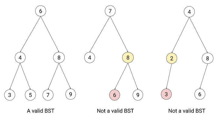
For more information, visit the source of the image.

Remark: Finding the node containing a given query key (or determining that no node contains the key, the maximum key or minimum key) can be done by traversing down the tree, recursively exploring the appropriate subtree.

Remark: The complexity of tree operations depends on the tree’s height rather than the number of items stored in it.

Returning to our problem, we will define algorithms to efficiently find the minimum or maximum and quickly insert or delete items in a binary search tree.

Minimum

A efficient way of finding the node associated to the minimum key in a BST is simply done by following the left child from the root until we encoutner a NIL value. The pseudo-code is given bellow:

TREE-MINIMUM(x)
1  while left[x] ≠ NIL
2      do x ← left[x]
3  return x

Remark: Observe that if binary search tree property is satisfied then TREE-MINIMUM(x) is correct (meaning that the minimum is found).

Remark: Observe also that the complexity of TREE-MINIMUM(x) is of order $O(h)$, where $h$ is the height of the tree.

You can think now on how to design TREE-MAXIMUM(x) which should return the node associated to the maximum key in a BST.

Insertion in BST

When we want to insert a key in a BST, one of the main difficulty is that we have to maintain the binary search property. The classical approach is to insert the new key at a leaf. To decide after which leaf the new key should be added, the following iterative procedure can be followed:

• If the new key is less than the current node move to the left subtree.
• Otherwise, move to the right subtree.

You can find the pseudo-code below:

TREE-INSERT(T, z)
1  y ← NIL
2  x ← root[T]
3  while x ≠ NIL
4      do y ← x
5         if key[z] < key[x]
6             then x ← left[x]
7             else x ← right[x]
8  p[z] ← y
9  if y = NIL
10     then root[T] ← z        ▷ Tree T was empty
11     else if key[z] < key[y]
12             then left[y] ← z
13             else right[y] ← z

A more detailed explaination: The variable x traces the path in the tree and y is the current parent of x. The while loop in lines 3-7 makes the two variables to move down the tree, going left or right depending on if the key of z is bigger or smaller than the key of the current node x. If x = NIL then a leaf has been reached. This leaf is where the item z is placed. The 8-13 set the variables to ensure that z is inserted in the right place in the tree.

Remark: TREE-INSERT(T, z) runs in $O(h)$, where $h$ is the height of the tree.