Machine Learning Techniques: From Theory to Practice

Duration1h AI Allowed

This course introduces the main families of machine learning techniques, including unsupervised learning, supervised learning, cross-validation, hyperparameter tuning, and model evaluation. It was prepared by IMT Atlantique for the Data Science Toolkit and Applications course.

Table of contents

1. Introduction to Machine Learning
2. Unsupervised Learning: Finding Hidden Patterns
3. Supervised Learning: Predicting the Future from the Past
4. Cross-Validation: Ensuring Robust Models
5. Hyperparameter Tuning: Fine-Tuning Your Model
6. Evaluation Metrics: Measuring Model Performance
7. Focus on P-value
8. Conclusion and Next Steps
9. Appendix: Cheat Sheets

1. Introduction to Machine Learning

1.1 What is Machine Learning?

Machine Learning (ML) is a subset of Artificial Intelligence (AI) that enables systems to learn from data and improve their performance over time without being explicitly programmed. It is a core component of Data Science, allowing us to build models that can:

• Predict future outcomes (e.g., stock prices, customer churn).
• Classify data into categories (e.g., spam vs. not spam, human vs. not human, dog/cat/bird/…).
• Cluster data into groups (e.g., customer similar profiles, ).
• Find patterns in complex datasets (e.g., association rules in retail).

1.2 Why is Machine Learning Important?

• Automation: Reduces the need for manual rule-based programming.
• Scalability: Handles large and complex datasets efficiently.
• Insights: Uncovers hidden patterns and relationships in data.
• Decision-Making: Provides data-driven insights for better business decisions.

1.3 Types of Machine Learning

There are several types of machine learning, each with special characteristics and applications. Some of the main types of machine learning algorithms are as follows:

• Supervised learning
• Unsupervised learning
• Reinforcement learning

Additional categories include semi-supervised and self-supervised learning, which combine elements of supervised and unsupervised approaches.

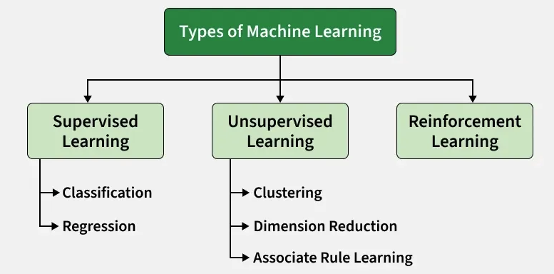
Figure 1: Types of machine learning.

2. Unsupervised Learning: Finding Hidden Patterns

2.1 Definition and Core Concepts

Unsupervised Learning is a type of ML where the model learns from unlabeled data (i.e., data without known outputs). The goal is to discover hidden patterns or groupings in the data.

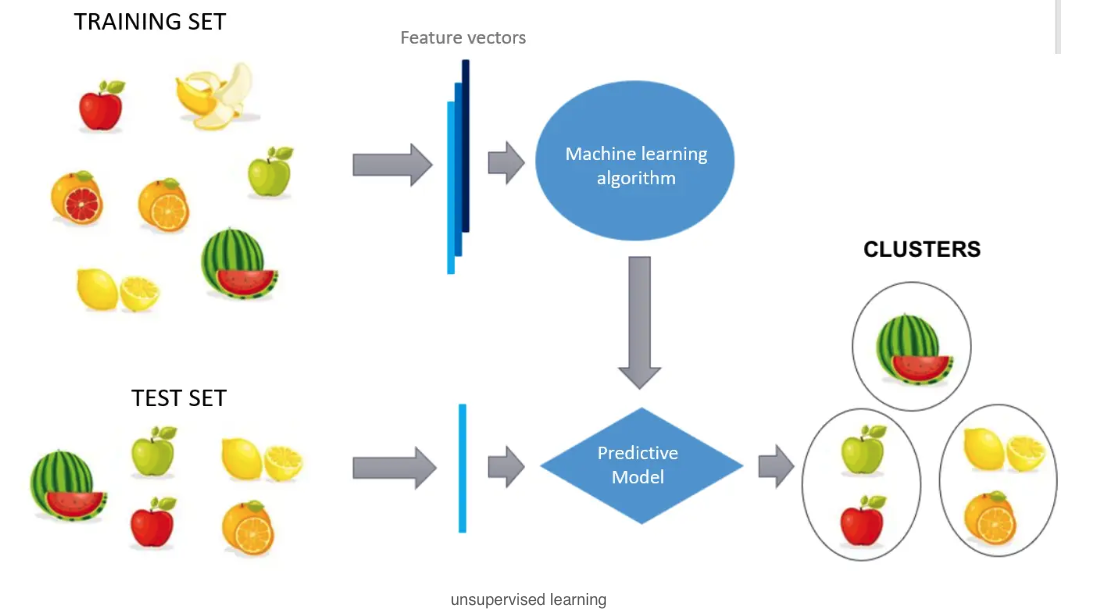
Key terminology

• Features (X): Input variables (same as supervised learning).
• Clusters: Groups of similar data points.
• Dimensionality Reduction: Reducing the number of features while preserving information.

2.2 Types of Unsupervised Learning Problems

2.3 Key Algorithms for Unsupervised Learning

2.3.1 Clustering Algorithms

K-Means Clustering

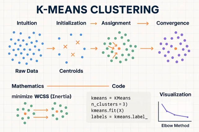
Partitions data into k clusters by minimizing the within-cluster variance.

How it works — Initialize k centroids, assign points to nearest centroid, recalculate centroids, repeat until convergence.

Pros Simple and fast, works well for spherical clusters.

Cons Requires choosing k, sensitive to outliers, assumes spherical clusters of similar size.

Use cases — Customer segmentation, image compression, document clustering.

DBSCAN (Density-Based Spatial Clustering of Applications with Noise)

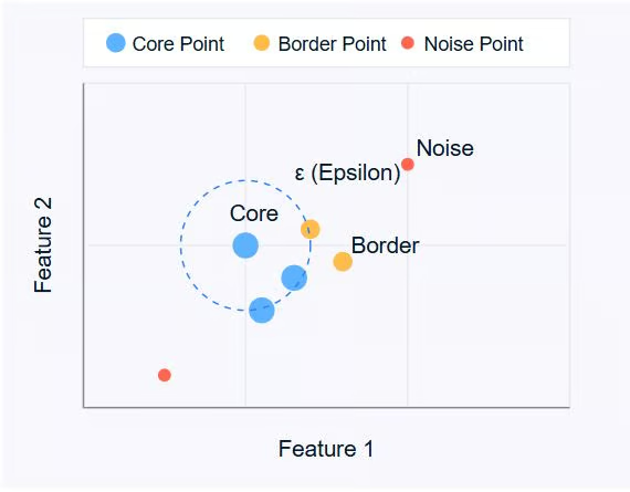
Groups data points that are close to each other (based on density) and marks outliers as noise.

Key Parameters — epsilon (ε, The maximum distance between two points for them to be considered as neighbors), min_samples (The minimum number of points required to form a dense region).

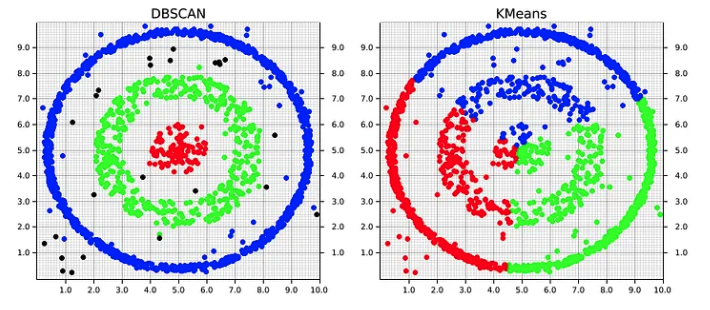
Pros No need to specify k, can find arbitrarily shaped clusters, robust to outliers.

Cons Sensitive to epsilon and min_samples, struggles with clusters of varying densities.

Use Cases — Anomaly detection, spatial data clustering, identifying dense regions in data.

Use K-Means when:

• You already know (or can estimate) the number of clusters.
• Clusters are compact and approximately spherical.
• The dataset contains few outliers.
• Speed is important. The dataset has many dimensions.

Use DBSCAN when:

• You do not know the number of clusters.
• You expect irregular cluster shapes.
• The data contain outliers or noise.
• You want to detect anomalies.
• Cluster membership should depend on local density.

2.3.2 Association Algorithms

Apriori Algorithm

Finds frequent itemsets and derives association rules from them.

Key Metrics — Support, Confidence, Lift.

Pros Simple and interpretable, works well for transactional data.

Cons Computationally expensive for large datasets, requires setting minimum support and confidence thresholds.

Use Cases — Market basket analysis, recommendation systems.

2.3.3 Dimensionality Reduction Algorithms

PCA (Principal Component Analysis)

Reduces the dimensionality of a dataset while preserving as much variance as possible.

Steps — Standardize data, compute covariance matrix, calculate eigenvectors, select top k eigenvectors, project data onto new subspace.

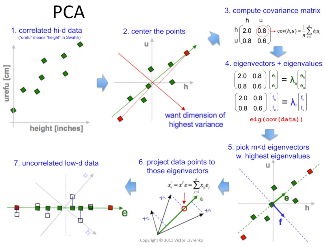
Pros Reduces noise and redundancy, speeds up machine learning algorithms, helps in visualizing high-dimensional data.

Cons Loss of interpretability, assumes linear relationships between variables.

Use Cases — Visualizing high-dimensional data, feature selection, data compression.

2.3.4 Code Examples for Unsupervised Learning

K-Means clustering example

 1
 2
 3
 4
 5
 6
 7
 8
 9
10
11
12
13
14
15
16
17

from sklearn.cluster import KMeans
from sklearn.datasets import load_iris
import matplotlib.pyplot as plt

iris = load_iris()
X = iris.data[:, :2]

kmeans = KMeans(n_clusters=3, random_state=42)
kmeans.fit(X)
y_pred = kmeans.predict(X)

plt.scatter(X[:, 0], X[:, 1], c=y_pred, cmap='viridis')
plt.scatter(kmeans.cluster_centers_[:, 0], kmeans.cluster_centers_[:, 1], marker='x', color='red', s=100)
plt.xlabel('Feature 1')
plt.ylabel('Feature 2')
plt.title('K-Means Clustering (k=3)')
plt.show()

DBSCAN example

 1
 2
 3
 4
 5
 6
 7
 8
 9
10
11
12
13

from sklearn.cluster import DBSCAN
from sklearn.datasets import make_moons
import matplotlib.pyplot as plt

X, _ = make_moons(n_samples=300, noise=0.05, random_state=42)
dbscan = DBSCAN(eps=0.3, min_samples=5)
y_pred = dbscan.fit_predict(X)

plt.scatter(X[:, 0], X[:, 1], c=y_pred, cmap='viridis')
plt.xlabel('Feature 1')
plt.ylabel('Feature 2')
plt.title('DBSCAN Clustering')
plt.show()

Apriori example using mlxtend

 1
 2
 3
 4
 5
 6
 7
 8
 9
10
11
12
13
14

# Install mlxtend if not already installed: pip install mlxtend
from mlxtend.frequent_patterns import apriori, association_rules
import pandas as pd

dataset = [['Milk', 'Onion', 'Nutmeg', 'Kidney Beans', 'Eggs', 'Yogurt'],
           ['Dill', 'Onion', 'Nutmeg', 'Kidney Beans', 'Eggs', 'Yogurt'],
           ['Milk', 'Apple', 'Kidney Beans', 'Eggs']]

te = pd.get_dummies(pd.DataFrame(dataset, columns=['Transaction']))
te = te.astype(int)

frequent_itemsets = apriori(te, min_support=0.5, use_colnames=True)
rules = association_rules(frequent_itemsets, metric="lift", min_threshold=1.0)
print(rules[['antecedents', 'consequents', 'support', 'confidence', 'lift']])

PCA example

 1
 2
 3
 4
 5
 6
 7
 8
 9
10
11
12
13
14
15

from sklearn.decomposition import PCA
from sklearn.datasets import load_iris
import matplotlib.pyplot as plt

iris = load_iris()
X = iris.data

pca = PCA(n_components=2)
X_pca = pca.fit_transform(X)

plt.scatter(X_pca[:, 0], X_pca[:, 1], c=iris.target, cmap='viridis')
plt.xlabel('Principal Component 1')
plt.ylabel('Principal Component 2')
plt.title('PCA: Dimensionality Reduction')
plt.show()

3. Supervised Learning: Predicting the Future from the Past

3.1 Definition and Core Concepts

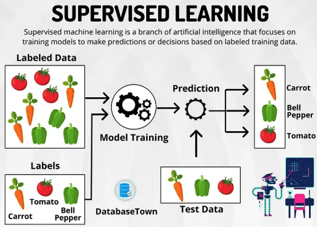
Supervised Learning is a type of ML where the model is trained on a labeled dataset (i.e., input data with known output labels). The goal is to learn a mapping from inputs to outputs so that the model can predict the output for new, unseen inputs.

Key terminology

• Features (X): Input variables (e.g., age, income, education).
• Label/Target (y): Output variable (e.g., “churn” or “no churn”).
• Training: The process of fitting the model to the labeled data.
• Prediction: Using the trained model to predict outputs for new inputs.

3.2 Types of Supervised Learning Problems

3.2.1 Classification

Goal: Predict a discrete label (category) for a given input. Examples: Spam detection (spam/not spam), medical diagnosis (disease/no disease), customer churn prediction (churn/no churn).

3.2.2 Regression

Goal: Predict a continuous value for a given input. Examples: House price prediction, sales forecasting, temperature prediction.

3.3 Key Algorithms for Supervised Learning

3.3.1 Classification Algorithms

Logistic Regression

A linear model for binary classification that uses the logistic function (sigmoid) to predict probabilities.

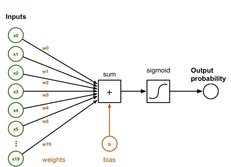
Pros Simple and interpretable, works well for linearly separable data, computationally efficient.

Cons Assumes linear relationship, sensitive to outliers, not suitable for complex non-linear relationships.

Use Cases — Binary classification (e.g., yes/no, true/false), risk assessment (e.g., loan approval).

Random Forest

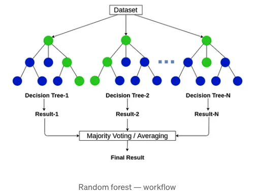
An ensemble learning method that builds multiple decision trees during training and outputs the mode (classification) or mean (regression) of the individual trees.

Pros Handles non-linear relationships well, robust to outliers and noise, works with high-dimensional data.

Cons Less interpretable than decision trees, can overfit if trees are too deep, slower than linear models for large datasets.

Use Cases — Classification (e.g., image recognition), regression (e.g., predicting house prices).

Support Vector Machines (SVM)

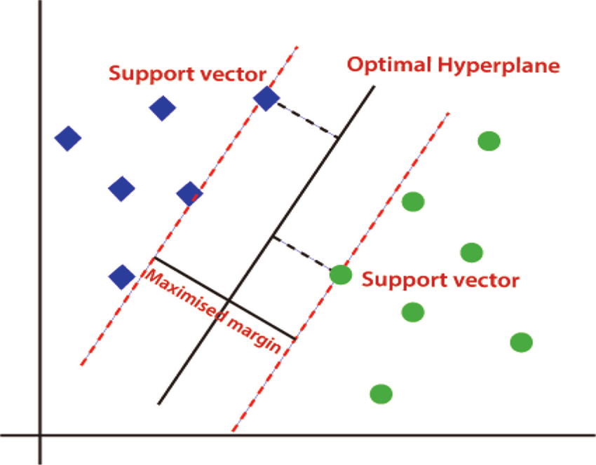
Finds the optimal hyperplane that best separates the classes in the feature space.

Key Concepts — Support Vectors, Margin, Kernel Trick.

Pros Effective in high-dimensional spaces, robust to overfitting, works well with small datasets.

Cons Sensitive to feature scaling, not ideal for large datasets, less interpretable than linear models.

Use Cases — Text classification, image recognition, bioinformatics.

3.3.2 Regression Algorithms

Linear Regression

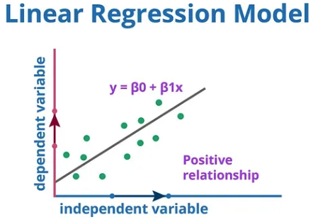
A linear approach to modeling the relationship between a dependent variable (target) and one or more independent variables (features).

Mathematical Formulation — $y = w_1x_1 + w_2x_2 + \cdots + w_nx_n + b$

Pros Simple and easy to interpret, fast to train, works well for linear relationships.

Cons Assumes linearity, sensitive to outliers, poor performance for non-linear data.

Use Cases — Predicting house prices, sales forecasting, trend analysis.

XGBoost (Extreme Gradient Boosting)

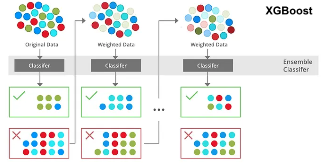
An ensemble learning method based on gradient boosting. Builds trees sequentially, where each new tree corrects the errors of the previous one.

Pros High performance, handles missing values automatically, robust to outliers.

Cons Complex to tune, slower than Random Forest for training, less interpretable.

Use Cases — Structured/tabular data, time-series forecasting, anomaly detection.

3.3.3 Code Examples for Supervised Learning

Logistic regression example

 1
 2
 3
 4
 5
 6
 7
 8
 9
10
11
12
13
14
15

from sklearn.linear_model import LogisticRegression
from sklearn.model_selection import train_test_split
from sklearn.metrics import accuracy_score, classification_report
from sklearn.datasets import load_breast_cancer

data = load_breast_cancer()
X, y = data.data, data.target
X_train, X_test, y_train, y_test = train_test_split(X, y, test_size=0.2, random_state=42)

model = LogisticRegression(max_iter=1000)
model.fit(X_train, y_train)
y_pred = model.predict(X_test)

print(f"Accuracy: {accuracy_score(y_test, y_pred):.2f}")
print(classification_report(y_test, y_pred))

Random Forest example

 1
 2
 3
 4
 5
 6
 7
 8
 9
10
11
12
13

from sklearn.ensemble import RandomForestClassifier
from sklearn.datasets import load_iris

data = load_iris()
X, y = data.data, data.target

model = RandomForestClassifier(n_estimators=100, random_state=42)
model.fit(X, y)

importances = model.feature_importances_
features = data.feature_names
for feature, importance in zip(features, importances):
    print(f"{feature}: {importance:.2f}")

4. Cross-Validation: Ensuring Robust Models

4.1 Definition and Core Concepts

Cross-Validation is a resampling technique used to evaluate machine learning models by partitioning the original dataset into training and validation subsets.

Why use cross-validation?

• Avoid Overfitting: Ensures the model performs well on unseen data.
• Better Estimate of Model Performance: Provides a more reliable estimate of the model’s generalization error.
• Optimal Use of Data: Maximizes the use of available data for both training and validation.

4.2 Techniques for Cross-Validation

4.2.1 Holdout Method

Splits the dataset into training set (typically 70-80%) and test set (typically 20-30%).

Pros Simple and fast, easy to implement.

Cons High variance in performance estimates, underutilizes data.

4.2.2 k-Fold Cross-Validation

Divides the dataset into k equal-sized folds. The model is trained on k-1 folds and validated on the remaining fold.

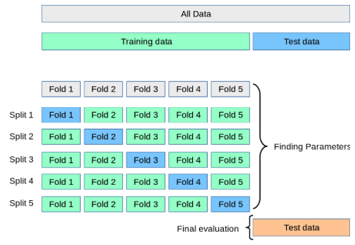
Pros Lower variance in performance estimates, maximizes data usage.

Cons Computationally expensive, not ideal for very large datasets.

4.2.3 GroupKFold Cross-Validation

• GroupKFold is used when samples are not independent because multiple observations belong to the same group.
• Its goal is to prevent data leakage by ensuring that all samples from a given group appear either in the training set or in the test set, but never in both.
• When to use GroupKFold: Use it whenever your dataset contains repeated measurements or related observations.

4.2.4 Stratified k-Fold Cross-Validation

A variant of k-fold that preserves the percentage of samples for each class in each fold.

Pros Handles imbalanced datasets well, provides a more reliable estimate for classification problems.

Cons Slightly more complex to implement than standard k-fold.

4.2.5 Code Examples for Cross-Validation

Holdout method example

 1
 2
 3
 4
 5
 6
 7
 8
 9
10
11
12
13

from sklearn.model_selection import train_test_split
from sklearn.ensemble import RandomForestClassifier
from sklearn.datasets import load_iris
from sklearn.metrics import accuracy_score

data = load_iris()
X, y = data.data, data.target
X_train, X_test, y_train, y_test = train_test_split(X, y, test_size=0.3, random_state=42)

model = RandomForestClassifier(random_state=42)
model.fit(X_train, y_train)
y_pred = model.predict(X_test)
print(f"Test Accuracy: {accuracy_score(y_test, y_pred):.2f}")

k-fold cross-validation example

 1
 2
 3
 4
 5
 6
 7
 8
 9
10
11
12

from sklearn.model_selection import KFold, cross_val_score
from sklearn.ensemble import RandomForestClassifier
from sklearn.datasets import load_iris

data = load_iris()
X, y = data.data, data.target
model = RandomForestClassifier(random_state=42)

kfold = KFold(n_splits=5, shuffle=True, random_state=42)
scores = cross_val_score(model, X, y, cv=kfold, scoring='accuracy')
print(f"Cross-Validation Scores: {scores}")
print(f"Mean Accuracy: {scores.mean():.2f} (±{scores.std():.2f})")

5. Hyperparameter Tuning: Fine-Tuning Your Model

5.1 Definition and Core Concepts

Hyperparameters are external configurations of a machine learning model that are not learned during training (e.g., number of trees in a Random Forest, learning rate in XGBoost). Hyperparameter tuning is the process of finding the optimal combination of hyperparameters to maximize model performance.

5.2 Techniques for Hyperparameter Tuning

5.2.1 Grid Search

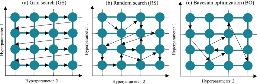
Exhaustively searches over a predefined set of hyperparameter values.

Pros Guarantees finding the best combination within the specified range, simple to implement.

Cons Computationally expensive, not feasible for large hyperparameter spaces.

5.2.2 Random Search

Randomly samples hyperparameter combinations from a predefined distribution.

Pros Faster than Grid Search for large spaces, often finds good combinations quickly.

Cons No guarantee of finding the best combination, may miss important regions of the hyperparameter space.

5.2.3 Bayesian Optimization

Uses probabilistic models (e.g., Gaussian Processes) to guide the search for optimal hyperparameters.

Pros More efficient than Grid/Random Search, can handle complex hyperparameter spaces.

Cons Complex to implement, requires more computational overhead per iteration.

5.2.4 Code Examples for Hyperparameter Tuning

Grid Search example

 1
 2
 3
 4
 5
 6
 7
 8
 9
10
11
12
13
14
15
16
17
18
19

from sklearn.model_selection import GridSearchCV
from sklearn.ensemble import RandomForestClassifier
from sklearn.datasets import load_iris

data = load_iris()
X, y = data.data, data.target

param_grid = {
    'n_estimators': [50, 100, 200],
    'max_depth': [None, 5, 10, 20],
    'min_samples_split': [2, 5, 10]
}

model = RandomForestClassifier(random_state=42)
grid_search = GridSearchCV(model, param_grid, cv=5, scoring='accuracy', n_jobs=-1)
grid_search.fit(X, y)

print(f"Best Hyperparameters: {grid_search.best_params_}")
print(f"Best Accuracy: {grid_search.best_score_:.2f}")

6. Evaluation Metrics: Measuring Model Performance

6.1 Evaluation Metrics for Classification

6.1.1 Confusion Matrix

6.1.2 Derived Metrics from Confusion Matrix

1. Accuracy

• Shows how many predictions the model got right out of all the predictions.
• It gives idea of overall performance but it can be misleading when one class is more dominant over the other.
• For example a model that predicts the majority class correctly most of the time might have high accuracy but still fail to capture important details about other classes.
• Formula: (TP + TN) / (TP + TN + FP + FN)
• When to Use: Balanced datasets.

2. Precision

• Precision focus on the quality of the model’s positive predictions.
• It tells us how many of the “positive” predictions were actually correct.
• It is important in situations where false positives need to be minimized such as detecting spam emails or fraud.
• Formula: TP / (TP + FP)
• When to Use: High cost of false positives.

3. Recall (Sensitivity or True Positive Rate)

• Recall measures how how good the model is at predicting positives.
• It shows the proportion of true positives detected out of all the actual positive instances.
• High recall is essential when missing positive cases has significant consequences like in medical tests.
• Formula: TP / (TP + FN)
• When to Use: High cost of false negatives.

4. F1-Score

• F1-score combines precision and recall into a single metric to balance their trade-off.
• It provides a better sense of a model’s overall performance particularly for imbalanced datasets.
• It is helpful when both false positives and false negatives are important though it assumes precision and recall are equally important but in some situations one might matter more than the other.
• Formula: 2 * (Precision * Recall) / (Precision + Recall)
• When to Use: Balance between precision and recall.

5. ROC Curve and AUC

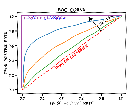
• The ROC curve gives a visual representation of the trade-offs between the true positive rate (TPR) and false positive rate (FPR) at various thresholds.
• ROC curve provides insights into how well the model can balance the trade-offs between detecting positive instances and avoiding false positives across different thresholds.
• AUC, or Area Under the Curve, is a single scalar value ranging from 0 to 1, that gives a performance snapshot of the model.
• You only calculate AUC after generating the ROC curve because the AUC represents the area beneath the curve.
• TPR (Recall): TP / (TP + FN)
• FPR: FP / (FP + TN)
• AUC: Area Under Curve (1.0 = perfect, 0.5 = random).

6.1.3 Code Example: Classification Metrics

 1
 2
 3
 4
 5
 6
 7
 8
 9
10
11
12
13
14
15
16
17
18
19
20
21

from sklearn.metrics import accuracy_score, precision_score, recall_score, f1_score, roc_auc_score, confusion_matrix, classification_report
from sklearn.datasets import load_breast_cancer
from sklearn.model_selection import train_test_split
from sklearn.ensemble import RandomForestClassifier

data = load_breast_cancer()
X, y = data.data, data.target
X_train, X_test, y_train, y_test = train_test_split(X, y, test_size=0.2, random_state=42)

model = RandomForestClassifier(random_state=42)
model.fit(X_train, y_train)
y_pred = model.predict(X_test)
y_proba = model.predict_proba(X_test)[:, 1]

print(f"Accuracy: {accuracy_score(y_test, y_pred):.2f}")
print(f"Precision: {precision_score(y_test, y_pred):.2f}")
print(f"Recall: {recall_score(y_test, y_pred):.2f}")
print(f"F1-Score: {f1_score(y_test, y_pred):.2f}")
print(f"ROC-AUC: {roc_auc_score(y_test, y_proba):.2f}")
print(f"Confusion Matrix:\n{confusion_matrix(y_test, y_pred)}")
print(f"Classification Report:\n{classification_report(y_test, y_pred)}")

6.2 Evaluation Metrics for Regression

6.2.1 Mean Absolute Error (MAE)

• Mean Absolute Error measures the average absolute difference between actual and predicted values.
• It treats all errors equally, regardless of their direction and provides results in the same unit as the target variable, making it easy to interpret.
• Formula: mean(|y_true - y_pred|)
• When to Use: Simple, interpretable metric.
• Interpretation example: MAE = 42.79: An MAE of 42.79 indicates that, on average, the model’s predictions deviate from the actual values by approximately 42.79 units.

6.2.2 Mean Squared Error (MSE)

• Mean Squared Error calculates the average of squared differences between actual and predicted values.
• By squaring errors, it penalizes larger mistakes more strongly, making it sensitive to outliers.
• Formula: mean((y_true - y_pred)²)
• When to Use: Penalizes large errors more heavily.
• Interpretation example: MSE=2900.19: An MSE of 2900.19 shows that the average of the squared prediction errors is 2900.19, meaning the model incurs some large errors that are heavily penalized.

6.2.3 Root Mean Squared Error (RMSE)

• Root Mean Squared Error is the square root of MSE.
• It maintains the strong penalty for large errors while converting the result back to the original unit of the target variable, improving interpretability.
• Formula: sqrt(MSE)
• When to Use: Same units as the target.
• Interpretation example: RMSE=53.85: An RMSE of 53.85 suggests that the model’s predictions typically differ from the actual values by about 53.85 units, in the same scale as the target variable.

6.2.4 R-Squared (R²)

• R-squared represents the proportion of variance in the target variable that is explained by the regression model.
• It provides insight into how well the model captures underlying data patterns.
• Formula: 1 - (SS_res / SS_tot)
• When to Use: Compare models, measure explanatory power.
• Interpretation example: R²=0.45: An R² value of 0.45 indicates that the model explains approximately 45% of the variance in the target variable, reflecting moderate predictive capability.

6.2.5 Code Example: Regression Metrics

 1
 2
 3
 4
 5
 6
 7
 8
 9
10
11
12
13
14
15
16

from sklearn.metrics import mean_absolute_error, mean_squared_error, r2_score
from sklearn.datasets import make_regression
from sklearn.model_selection import train_test_split
from sklearn.linear_model import LinearRegression

X, y = make_regression(n_samples=100, n_features=1, noise=10, random_state=42)
X_train, X_test, y_train, y_test = train_test_split(X, y, test_size=0.2, random_state=42)

model = LinearRegression()
model.fit(X_train, y_train)
y_pred = model.predict(X_test)

print(f"MAE: {mean_absolute_error(y_test, y_pred):.2f}")
print(f"MSE: {mean_squared_error(y_test, y_pred):.2f}")
print(f"RMSE: {mean_squared_error(y_test, y_pred, squared=False):.2f}")
print(f"R²: {r2_score(y_test, y_pred):.2f}")

6.3 Evaluation Metrics for Clustering

6.3.1 Silhouette Score

• Formula: (b - a) / max(a, b)
  • a = Average distance between a sample and all other points in the same cluster.
  • b = Average distance between a sample and all other points in the nearest cluster.
• When to Use: Evaluate clustering quality.

6.3.2 Davies-Bouldin Index

• Formula: Average ratio of intra-cluster distance to inter-cluster distance.
• When to Use: Compare clustering algorithms.

6.3.3 Code Example: Clustering Metrics

 1
 2
 3
 4
 5
 6
 7
 8
 9
10
11
12
13

from sklearn.metrics import silhouette_score, davies_bouldin_score
from sklearn.cluster import KMeans
from sklearn.datasets import load_iris

data = load_iris()
X = data.data

kmeans = KMeans(n_clusters=3, random_state=42)
kmeans.fit(X)
y_pred = kmeans.predict(X)

print(f"Silhouette Score: {silhouette_score(X, y_pred):.2f}")
print(f"Davies-Bouldin Index: {davies_bouldin_score(X, y_pred):.2f}")

7. Focus on P-value

7.1 Core concept

A p-value (probability value) is a statistical measure used in hypothesis testing to help decide whether the results of an experiment are meaningful or likely due to random chance.

• It represents the probability of observing results as extreme as the ones obtained assuming the null hypothesis $H_0$ is true.
• In simple terms it answers the question “If nothing unusual is happening, how surprising are these results?”
• A small p-value means the observed results are unlikely to occur by chance alone providing strong evidence against the null hypothesis.
• A large p-value suggests the results are consistent with random variation and do not provide enough evidence to reject the null hypothesis.

If we have a target variable (the case in regression for example), the p-value helps answer the question: “Is this predictor truly associated with the target, or could the observed relationship be due to random chance?”

Where to use: P-value can be used in several cases

• Pre-processing and Feature Selection in Modeling: During model training, p-values help identify variables that significantly impact predictions.
• Medical Research: P-values are widely used to determine whether a drug or treatment has a significant effect on patients.
• Business Decision Making: In business analytics p-values help evaluate whether observed trends or patterns are statistically significant aiding informed decisions.
• Quality Control: P-values are used in manufacturing to check if variations in production are due to random chance or indicate a real problem.
• Social Science Research: Researchers use p-values to confirm if observed effects are significant.

7.2 Interpretation example

Suppose a regression output is:

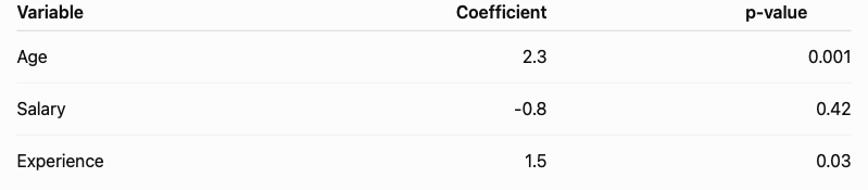
Age (p = 0.001)

• Very strong evidence against $H_0$
• Age is statistically associated with the target.

Salary (p = 0.42)

• Weak evidence against $H_0$
• We fail to reject $H_0$ .
• There is insufficient evidence that Salary contributes after accounting for the other variables.
• Note: “Fail to reject” is not the same as proving there is no effect. It means the data do not provide enough evidence for a non-zero effect.

Experience (p = 0.03)

• Significant at the 5% level.
• Experience likely has a real association with the target.

7.3 Common significance levels

7.4 Important misconceptions

❌ “A p-value of 0.03 means there’s a 97% chance the variable is important.”

• Incorrect.
• A p-value is not the probability that the null hypothesis is true.
• It is:“Assuming the coefficient is truly zero, how surprising would the observed data be?”

❌ “A small p-value means the effect is large.”

• Incorrect.
• The p-value measures evidence, not effect size.

Example: coefficient versus p-value

7.5 Interpret p-values alongside the coefficient estimate

A p-value tells you whether there is statistical evidence of an effect, but it does not tell you how large or important that effect is. That’s why you should always interpret it together with the coefficient estimate.

Consider the linear regression model: $y = \beta_0 + \beta_1 x_1 + \cdots + \beta_n x_n$

For each predictor, the regression output provides:

• Coefficient estimate $\hat{\beta}$: the estimated effect size.
• p-value: the evidence that the true coefficient differs from zero. These answer different questions:

Example

7.6 When can p-values be misleading?

A statistically significant p-value does not guarantee that the result is practically meaningful. Be cautious when:

• Sample size is very large: Even tiny, practically irrelevant effects can produce very small p-values.
• Predictors are highly correlated (multicollinearity): Standard errors increase, making truly relevant variables appear non-significant.
• Model assumptions are violated: Ordinary least squares inference assumes linearity, independent errors, constant error variance (homoscedasticity), and approximately normal residuals for small samples. Violations can make p-values unreliable.
• Many predictors are tested simultaneously: Some small p-values can occur by chance (multiple testing).

8. Conclusion and Next Steps

8.1 Key Takeaways

8.2 Resources for Further Learning

Books

• Hands-On Machine Learning with Scikit-Learn, Keras, and TensorFlow by Aurélien Géron
• The Hundred-Page Machine Learning Book by Andriy Burkov

Online courses

• Machine Learning (Coursera) by Andrew Ng
• Data Science MicroMasters (edX) by UC San Diego

Tools and libraries

• Scikit-learn
• TensorFlow
• PyTorch
• XGBoost
• Pandas

Datasets for practice

• Kaggle Datasets
• UCI Machine Learning Repository

8.3 Next Steps

• Learn about advanced fields: Deep Learning, NLP, or Reinforcement Learning.
• Learn Cloud Tools: Google Vertex AI, AWS SageMaker, or Azure Machine Learning.
• Contribute to Open Source: Scikit-learn, TensorFlow, or PyTorch on GitHub.

9. Appendix: Cheat Sheets

9.1 Supervised Learning Cheat Sheet

9.2 Unsupervised Learning Cheat Sheet

9.3 Cross-Validation Cheat Sheet

9.4 Hyperparameter Tuning Cheat Sheet

9.5 Evaluation Metrics Cheat Sheet

Knowledge Check

Answer these questions after reading the lesson. Use the feedback to identify which concepts you should review before starting the practical activities.