Query Execution Process
What happens when an SQL query is submitted to a Relational DB Management System (RDBMS)? The goal of this document is to detail and analyse the different steps your query goes through to obtain its result. A focus is put on the way Postgresql executes a query but most of the existing RDBMS behave similarly.
Query execution steps
When an SQL query (e.g., SELECT * FROM users WHERE age > 30;) is submitted, the RDBMS has to analyse the query to determine the best way to access the data and to return the result. The execution pipeline typically involves the following steps:
- Parsing
- Validation
- Logical optimization
- Physical optimization (plan selection)
- Execution
- Returning results
Let us consider the following toy DB:
|
|
And now, you shall find below how the following query is executed step-by-step:
|
|
Parsing
The parser checks syntax and converts the SQL text into a parse tree.
|
|
Validation
The system checks:
- table existence (users, cities)
- column names (name, age, city_id)
- join compatibility (INT = INT)
- user permissions
This step builds a so-called validated query tree where now each identifier is resolved to an internal object reference:
|
|
Logical Optimisation
The optimizer rewrites the query using relational algebra rules.
σ(age > 30) (users ⋈ cities) is rewritten into (σ(age > 30) users) ⋈ cities indicating that the selection on users is performed before the join with the table cities.
It leads to an optimized query tree:
|
|
Physical Optimisation
The optimizer checks the stored meta-data about the data distribution in the so-called *statistics DB and also checks the presence of indexes.
Assume for instance that:
users(age)has an indexcities(id)is primary keyusershas 1,000,000 rowscitieshas 10,000 rows
The optimizer then might decide to retrieve data following the physical plan:
|
|
Execution
The optimised execution plan is then executed row-by-row. To effectively retrieve the stored data, the storage engine is used. It determines how to use buffers to load data pages, to lock tables to avoid concurrency access, etc.
For our running example:
- Index seek on users.age > 30 → access 30–40 pages
- For each users row:
- Seek on cities.id → access 1 page per lookup (likely cached)
Returning results
The execution streams the answers to the client to get the resulting table.
Summary of the execution process
|
|
Query execution plan
The EXPLAIN keyword placed in front of an SQL SELECT query outputs the query execution plan that will be used to calculate the query result.
Combined with ANALYZE keyword you also get the runtime measurements.
Here is an example of a basic SQL query:
|
|
And its possible execution plan:
|
|
An execution plan is tree of operators executed from the leaves to the root noe. A leaf generally leads to a table or index scan to retrieve the concerned tuples and an internal node is a join, sort or aggregation. The root node produces the result.
In the previous example, PostgreSQL gets rows from users (via index), then for each row, it probes cities (also via index) and finaly combines rows and outputs them:
|
|
Cost estimation
Between parenthees, the cost per operation is also given in the following format (cost=STARTUP..TOTAL rows=ESTIMATED width=AVERAGE_ROW_SIZE):
STARTUPindicates time before the first answer (i.e. tuple) is retrieved,TOTALis the estimated cost to output all answers (i.e. the complete result),rowsis an estimation, based DB statistics, of the number of tuples forming the result,widthis the size in byte of each returned tuple, it depends on the number of attributes on which it is projected. The time is not necessary in second, it can be in any unit as disk I/O operations, CPU operations, etc.
When ANALYZE is indicated, you also get the actual cost of each node. It also indicates the time to get the first tuple, all tuples, the number of tuples and the number of times (loops) the node is executed. Using nested loops, a same internal node will be executed several times.
The last lines of the execution plan recap the total time (in millisecond) taken by the planner (parsing, validating, and optimizing the query) and the overall execution time.
Internal node
An internal node in a query execution plan may refer to one of the following operators (only the main operators are described) :
-
seq scan when there is no other choice than scanning the whole table to identify the tuples satisfying the condition.
-
Index Scan Uses a B-Tree index; returns rows in index order.
-
Index Only Scan Reads only the index (no table access) when all needed columns exist in the index.
-
Bitmap Index Scan Builds a bitmap of matching row locations (TIDs), later consumed by a bitmap heap scan.
-
Bitmap Heap Scan Visits actual table pages using the bitmap built by bitmap index scans.
-
Nested loop when each row of the outer side has to be joined to a tuple for the inner side (ex. joining each user to its city). This kind of operation is selected when the number of tuples in the outer side is low and looking up to the inner tuples to associate with is fast (presence of an index).
-
Hash Join Builds a hash table from the smaller input; probes it with the larger one.
-
Merge Join Requires both inputs sorted on join key. Fast for already-sorted inputs (e.g., from an index scan).
-
Sort Performs an internal sort (in memory or on disk).
-
Incremental Sort Optimized sort for partially sorted inputs.
-
Unique Removes duplicates after a sort or merge join.
-
Aggregate (GroupAggregate) Classic group-by implemented by sorting + grouping.
-
HashAggregate Uses a hash table to group rows; faster for large groups not fitting in memory.
Used for UNION, INTERSECT, EXCEPT.
- Append Concatenates results of multiple subplans (e.g., UNION ALL).
- Merge Append Merges sorted inputs into a sorted output.
- SetOp Implements INTERSECT, EXCEPT, UNION DISTINCT.
Take-away message about execution plan
- Costs are estimates, times are real
- EXPLAIN ANALYZE is always preferred.
- Large differences between estimated rows and actual rows
- indicates bad statistics or poor index choices, a refresh of the DB statistics is needed.
- loops > 1
- indicates nested-loop behavior.
- Watch for these performance red flags:
- Seq Scan on very large tables
- Hash Join with huge hash table builds
- Sort on large inputs without work_mem
- Misestimated rows leading to wrong plan choices
- The plan reads bottom-up
- Scans → Filters → Joins → Aggregates → Sorts → Output
A focus on DB Statistics
As seen in the previous section, the query execution engine has to estimate the cost of each operator. To decide the best query execution strategy, it is crucial to estimate the number of tuples satisfying a selection criteria (e.g. users.age > 30).
To make these estimations, RDBMSs maintain statistics (using the auto-vacuum process or manually using the ANALYZE; query) about the tuples values distribution on each attribut domain.
In Postgresql, these statistics are stored in tables of the catalog DB. One can access these statistics through the pg_stats table. For instance, the following query:
|
|
returns the ratio of null values (null_frac), the number of distinct values (n_distinct), the most common values (most_common_vals), their frequencies (most_common_freqs), the bounds of the histogram (histogram_bounds) and correlation with other attributes (correlation).
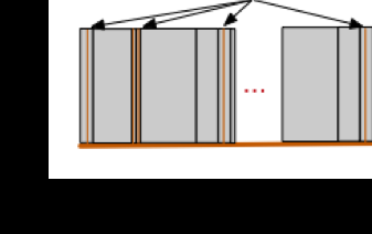
In case of a numerical attribute, Postgresql maintains an equi-height histogram. The domain is divided in buckets (by-default 100), each bucket defining a domain interval and they all cover the same amount of tuples. The figure below illustrates such equi-height histogram. Postgresql assumes that, within the interval, the tuples follow a normal distribution. In addition, Postgresql maintains a list of the 100 most frequent values and their associated number of occurences.
In case of a categorical value, Postgresql maintains only a table of the most frequents values (100 by default) and their respective frequency. It then considers again a normal distribution of the over values on the rest of the domain.