Algorithmic complexity

In brief

Article summary

Algorithmic complexity is a fundamental notion in computer science. It allows to characterize an algorithm, and provide an estimate of its needed time to complete, as a function of its inputs. This allows to evaluate if a problem can be solved in reasonable time, but also to compare multiple algorithms that solve a single problem. Besides, this is a measure that does not depend on the quality of your CPU, as it needs not the program to be run.

Main takeaways

• Algorithmic complexity estimates the needed time for an algorithm to complete.

• Complexity is expressed as a function of the input size.

• There are classes of complexity.

• We are generally interested in worst-case complexity, but other measures exist.

Article contents

1 — Algorithmic complexity

The goal of any algorithm is to propose a solution to a given problem. Minimizing the processing time is directly related to the number of calculations involved.

Algorithm complexity is a measure of the performance of a program in terms of the number of calculations it performs. The lower the algorithmic complexity, the fewer calculations the algorithm performs, and the higher its performance.

Loops are the main cause of the large number of calculations. Their uncontrolled use leads to an increasing number of operations. Beyond a certain number, the computation time becomes an obstacle to the use of the program. It is therefore important to be able to evaluate the performance of an algorithm before programming it.

2 — Analysis of complexity

There are several methods of complexity analysis, including:

• Average analysis provides information about the average computation time.
• Pessimistic analysis (worst-case) is the most commonly used. It provides information about the number of computations to be considered in a worst-case scenario. Its main purpose is to evaluate algorithms at their most extreme.

For example, if an algorithm searches for a data item among $N$ initial data items, in the worst case all data items, the pessimistic analysis will indicate that the search makes $N$ comparisons. The algorithmic complexity is then denoted as $O(N)$. The notation $O(\cdot)$ indicates that the performance analysis focuses on the upper bound. The value $N$ indicates that a maximum of $N$ processing operations must be performed when there is $N$ initial data.

3 — Main categories of complexity

Complexity varies from one algorithm to another, but can be grouped into the following categories:

3.1 — Logarithmic algorithms

Their notation is $O(log(N))$. These algorithms are very efficient in terms of processing time. The number of calculations depends on the logarithm of the initial number of data to be processed. The $log(N)$ function has a curve that flattens out horizontally as the number of data increases. The number of calculations increases slightly as the amount of data to be processed increases (see figure below).

Logarithmic algorithms process the dataset by dividing it into two equal parts, then repeating the process on each half. This is the logarithm in base 2, $log_2(N)$. To simplify writing the complexity of these algorithms, the notation $log(N)$ is used instead of $log_2(N)$.

3.2 — Linear algorithms

Their notation is of the form $O(N)$. They are fast algorithms. The number of calculations depends linearly on the number of initial data to be processed.

3.3 — Linear and logarithmic algorithms

Their notation is of the form $O(N \cdot log(N))$. They are algorithms that repeatedly divide a set into two parts and iterate through each part completely.

3.4 — Polynomial algorithms

Their notation is of the form $O(N^p)$, where $p$ is the power.

3.5 — Exponential or factorial algorithms

Their notation is of the form $O(e^N)$ or $O(N!)$. These are among the most complex algorithms. The number of calculations increases exponentially or factorially depending on the data being processed.

4 — Summary

Visually, we can understand the relatonships between complexities as follows:

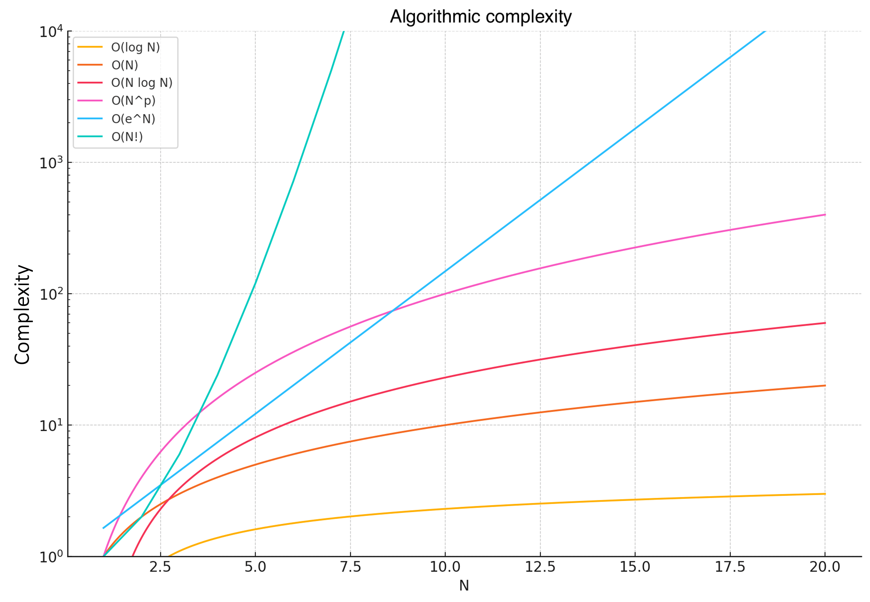
The curves clearly show how each complexity function grows with increasing $N$.

• $O(log(N))$ – Very slow curve growth (low complexity).
• $O(N)$ – Linear curve growth.
• $O(N \cdot log(N))$ – Slightly faster curve growth.
• $O(N^2)$ – Quadratic growth.
• $O(e^N)$ – Exponential growth (very high complexity).
• $O(N!)$ – Factorial growth (extremely high complexity).

Although memory management is not included in the notion of complexity, it often depends on it. It is common to use more memory to minimize the number of operations. We therefore need to check that the memory management of high performance algorithms does not become a new constraint on their use.

To go further

To go beyond

• name.

  Short description.