Practical session
Duration1h40Presentation & objectives
In this practical activity, we guide you through a first usage of machine learning tools. We will rely on data in matrix form, and will implement both a $k$-NN and a $k$-means algorithms. Later, in programming session 5, we will rely on existing libraries for more efficiency.
The aim of this session is to help you master important notions in computer science. An intelligent programming assistant such as GitHub Copilot, that you may have installed already, will be able to provide you with a solution to these exercises based only on a wisely chosen file name.
For the sake of training, we advise you to disable such tools first.
At the end of the practical activity, we suggest you to work on the exercise again with these tools activated. Following these two steps will improve your skills both fundamentally and practically.
Also, we provide you the solutions to the exercises. Make sure to check them only after you have a solution to the exercises, for comparison purpose! Even if you are sure your solution is correct, please have a look at them, as they sometimes provide additional elements you may have missed.
Activity contents
1 — Data Preparation
The goal of this first exercise is to:
- Familiarize yourself with dealing with multidimensional data.
- Generate a synthetic dataset composed of clouds of points.
- Split this dataset into a training set and a test set.
For this, we will use the numpy package in Python.
1.1 — How to create arrays
Numpy proposes multiple functions to build arrays:
- Creating arrays with
np.array(),np.zeros(),np.ones(),np.arange(). - Use the
np.shape()function on anynumpyarray to know its shape (numbers of rows, columns, etc.).
The np.array() function converts a Python list (or a list of lists) into a numpy array.
You can also create arrays filled with zeros or ones using np.zeros() and np.ones().
Here are a few examples of how to define arrays in Python using numpy:
# Needed imports
import numpy as np


# Creating a 1D array from a list
array_1d = np.array([1, 2, 3, 4, 5])
print("1D Array:", array_1d)

# Creating a 2D array (list of lists)
array_2d = np.array([[1, 2, 3], [4, 5, 6], [7, 8, 9]])
print("2D Array:\n", array_2d)

# Creating a 1D array of zeros
zeros_1d = np.zeros(5)
print("1D Array of zeros:", zeros_1d)

# Creating a 2D array (3 rows, 4 columns) of zeros
zeros_2d = np.zeros((3, 4))
print("2D Array of zeros:\n", zeros_2d)

# Creating a 2D array (2 rows, 3 columns) of ones
ones_2d = np.ones((2, 3))
print("2D Array of ones:\n", ones_2d)
print(np.shape(ones_2d))
Once numpy arrays have been defined, you can access their values (or groups of values), using square brackets, like lists, but separating dimensions using commas (,).
You can also use the colon (:) to select all elements of a dimension, and use negative integers to count backwards.
Illustration with a few useful indexing examples:
# Once numpy arrays have been defined, you can access their values (or groups of values), using square brackets, like lists, but separating dimensions using `,`.
print("Array1D: " , array_1d)
print("Array2D: " , array_2d)

# Accessing elements of a 1D array
print("Element of array1d at index 0:", array_1d[0])
print("Element at array1d at index 1:", array_1d[1])

# Accessing elements of a 2D array
print("Element of array2d at 0, 0:", array_2d[0, 0])
print("Element at array2d 0, 1:", array_2d[0, 1])

# Accessing all elements of a row
print("All elements of array2d row 0:", array_2d[0])
print("All elements of array2d, column 0: ", array_2d[:,0])

# Accessing the last row
print("Elements of last row:", array_2d[-1])
print("Element at last row, second column:", array_2d[-1, 1])
print("Elements of second to last column:", array_2d[:,-2])

# It is also possible to use an array of booleans (`True` or `False`, or ones and zeros) in order to select specific rows / columns

# Select elements that are greater than 2, and get their indices
print(f"Elements greater than 2: {array_1d[array_1d > 2]}, at indices {np.where(array_1d > 2)}")

# Use a vector of indices to select specific elements
print("Elements at 0, 2, 4 of array_1d:", array_1d[[0, 2, 4]])
A more complete tutorial on indexing can be found here: numpy tutorial on indexing.
Finally, it is also possible to generate random arrays using numpy, with functions np.random.normal(), np.random.uniform(), np.random.randint().
1.2 — Synthetic data generation
Using these functions, generate a synthetic dataset:
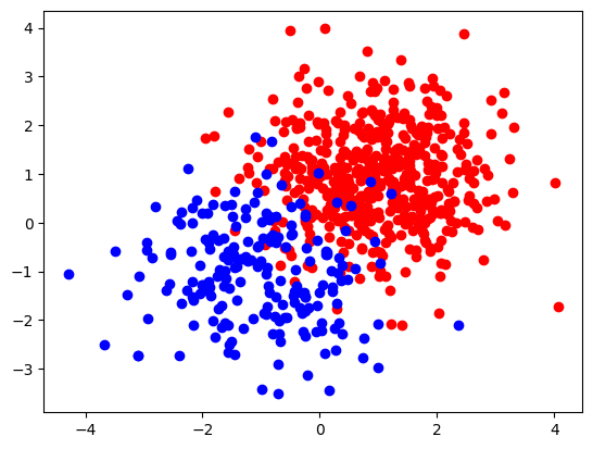
cloudAandcloudB, two clouds (sets) of points in dimension 2, following a normal distribution centered around around two distinct coordinates (coord1_Aorcoord1_B) with variance 1 (coord2_Aorcoord2_B).- Che number of points to generate in each cloud is given,
N_A = 500andN_B = 200.
Here is a visualisation of the two clouds (assuming that you named the two could points cloudA and cloudB)
as a scatter plot using the matplotlib library.
# Needed imports
import matplotlib.pyplot as plt


# Plot the clouds
plt.scatter(cloudA[:, 0], cloudA[:, 1], c='r')
plt.scatter(cloudB[:, 0], cloudB[:, 1], c='b')

# Display all open figures
plt.show()

1.3 — Prepare the dataset and split into a training and test set
We will now prepare the dataset. The following steps are needed:
- For each cloud, prepare a vector of labels, using a different integer value for each, for instance
0for cloud A and1for cloud B. - Using the
np.vstackand/ornp.hstackfunction (vertical/horizontal stack), concatenate the two clouds into one arrayXand the labels vector into a (1D) arrayy. - Generate a vector of permutations of the indices of the concatenated array using
np.random.permutation(). - Use this permutation to split
XandyintoX_train,y_trainandX_test,y_testwith ratios 80 percent for train / 20 percent for test. - Check the shapes of the generated train and test set.
vstack, hstack
np.random.permutation
2 — Supervised learning using $k$-nearest neighbors
In this exercice, we will implement the prediction on a test dataset using a $k$-NN on a training dataset. You can have a look at the course material to understand the principle of the algorithm. The different steps of the $k$-NN are as follows.
For each sample in the test dataset:
- Compute all pairwise distances between the sample and the training dataset.
- Extract the labels of the k smallest distances.
- Assign the label according to the one that is the most represented in the labels associated to the $k$ smallest distances (majority vote).
We will use the Euclidean distance to consider distances between samples. You can test your function on the train / test dataset generated in the first part.
The function should have the following signature:
# Needed imports
import numpy as np
from typing import List


def kNN (k: int, X_train: np.array, y_train: List[int], X_test: np.array) -> np.array:

    """
        k-NN prediction on a test set using a training dataset.
        In:
            * k:       Number of neighbours to consider.
            * X_train: Training dataset, numpy array with N (samples) rows and d (features) columns.
            * y_train: List of N labels associated with each example in X_train.
            * X_test:  Test dataset, numpy array with M (samples rows and d (features) columns.
        Out:
            * List of M labels associated with each example in X_test according to the k nearest neighbours with X_train.
    """

    pass
Test your function with k = 3 using the train and test datasets you generated in the previous part.
You can use the following snippet to check the accuracy of the trained $k$-NN. Accuracy corresponds to the proportion of correct answers.
# Percentage of correct predictions
accuracy = np.mean(predictions == y_test)
print(f"Accuracy of k-NN with k={k}: {accuracy}")
Using the parameters that generate the dataset from the correction above, you should obtain an accuracy of approximately 0.93.
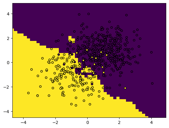
You can also plot decision boundaries using this snippet. This shows the areas that, according to the positions of the training points, will be classified as class A or B.
# Needed imports
from matplotlib.colors import ListedColormap
import numpy as np


def plot_boundaries (classifier, X, Y, h=0.2):

    # Create color maps
    x0_min, x0_max = X[:, 0].min() - 1, X[:, 0].max() + 1
    x1_min, x1_max = X[:, 1].min() - 1, X[:, 1].max() + 1
    x0, x1 = np.meshgrid(np.arange(x0_min, x0_max, h), np.arange(x1_min, x1_max, h))
    dataset = np.c_[x0.ravel(), x1.ravel()]
    Z = kNN(k, X, Y, dataset)

    # Put the result into a color plot
    Z = Z.reshape(x0.shape)
    plt.figure()
    plt.pcolormesh(x0, x1, Z)

    # Plot also the training points
    plt.scatter(X[:, 0], X[:, 1], c=Y, edgecolor='k', s=20)
    plt.xlim(x0.min(), x0.max())
    plt.ylim(x1.min(), x1.max())

    # Display the plot
    plt.show()


# Call the function with your training set
plot_boundaries(predictions, X_train, y_train)

3 — $k$-means clustering
In this exercise, we will implement the $k$-means algorithm from scratch. You can have a look at the course material) to understand the principle of the algorithm.
The different steps of $k$-means are as follows:
- Randomly initialize the centroids
- Compute current assignation of clusters.
- Update the centroids.
- Compute the current goodness of fit (GoF).
- Repeat from step 2 until convergence (GoF small enough).
The function should have the following signature:
from typing import List, Tuple

def k_means (k: int, X_train: np.array, X_test: np.array,max_iters:int, tol: float) -> Tuple[np.array, np.array]:

    """
        Cluster assignments on a test set according to clusters defined using k-means clustering on a training dataset.
        In:
            * k:         Number of clusters to consider.
            * X_train:   Training dataset, numpy array with N (samples) rows and d (features) columns.
            * X_test:    Test dataset, numpy array with M (samples rows and d (features) columns.
            * max_iters: Maximum number of iterations to run the k-means algorithm.
            * tol:       Convergence tolerance for centroid changes.
        Out:
            * List of M cluster assignements associated with each example in X_test.
            * Cluster centroids as a numpy array.
    """

    pass
Test your function with k = 2 using the train and test datasets you generated.
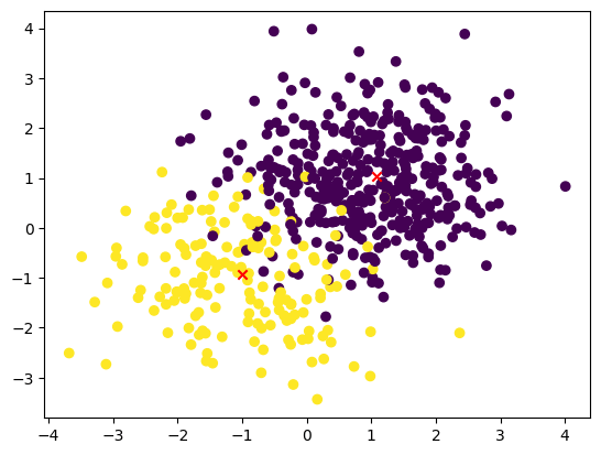
Use this code to visualize the dataset with the added cluster centroids.:
# Needed imports
import matplotlib.pyplot as plt

## Plot
plt.scatter(X_train[:, 0], X_train[:, 1], c=y_train)
plt.scatter(centroids[:, 0], centroids[:, 1], c='r',marker ='x')

5 — Optimize your solutions
What you can do now is to use AI tools such as GitHub Copilot or ChatGPT, either to generate the solution, or to improve the first solution you came up with! Try to do this for all exercises above, to see the differences with your solutions.
To go further
6 — Confusion matrix and performance metrics
You can further analyze the performance of a supervised learning algorithm using other tools:
-
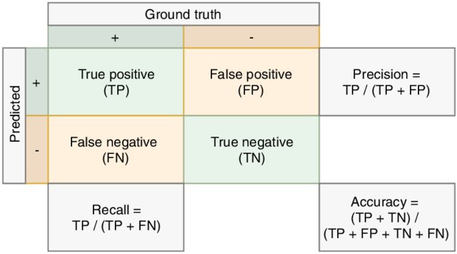
The confusion matrix is a (normalized) count of samples according to all occuring possibilities of predicted classes and true classes. Therefore it provides details on misclassifications, showing which classes are more difficult than others. You can estimate the confusion matrix using the confusion_matrix function from sklearn.
-
The precision score is the percentage of correctly classified examples with respect to all retrieved examples.
-
The recall score is the percentage of correctly classified examples with respect to all examples belonging to a given class.
-
The f1 score is the harmonic mean of precision and recall.
Here is an illustration of precision and recall:

These three metrics can be computed from the functions in the sklearn.metrics module.
An easy way to show all of them is to print the classification report.
To go beyond
Looks like this section is empty!
Anything you would have liked to see here? Let us know on the Discord server! Maybe we can add it quickly. Otherwise, it will help us improve the course for next year!