Parcours de graphes

Bonjour ! Et bienvenue dans cette leçon sur le parcours de graphes.

Trouver la sortie d’un labyrinthe nécessite de parcourir une partie du labyrinthe. Le parcours de graphes est le domaine de la théorie des graphes qui décrit comment explorer un graphe, un sommet à la fois, en partant d’un sommet initial.

Dans de nombreux cas, nous nous intéressons à l’atteignabilité. L’atteignabilité consiste à trouver comment atteindre un sommet cible à partir d’un sommet initial, en suivant un chemin dans le graphe.

Pour obtenir des chemins depuis le sommet initial vers tous les sommets atteignables, je vais vous montrer comment construire un arbre, obtenu à partir du graphe initial, qui contiendra juste assez d’informations pour nous guider vers n’importe quel sommet atteignable depuis le sommet initial.

Rappelons qu’un graphe est un couple $G$ composé d’un ensemble de sommets $V$ et d’un ensemble d’arêtes $E$. Nous devons maintenant définir quelques notions supplémentaires.

Nous définissons les voisins de $u$ dans $G$ comme l’ensemble des sommets $v$ tels que $\{u,v\}$ appartient à $E$.

Comme nous l’avons vu dans la leçon précédente, un arbre est un graphe connexe sans cycles.

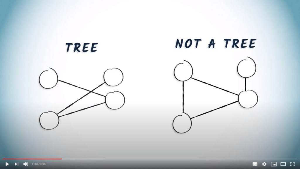
Par exemple, à gauche se trouve un dessin d’un arbre. Cependant, le graphe à droite n’est pas un arbre, car il contient un cycle.

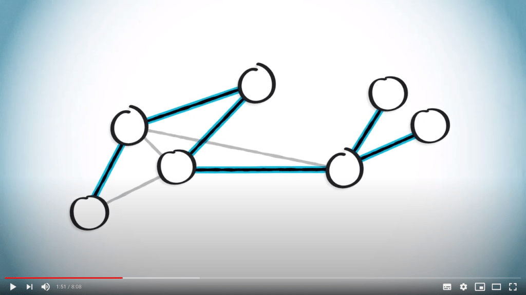
Un arbre couvrant d’un graphe $G$ est un arbre obtenu à partir de $G$ en supprimant certaines arêtes. Pour illustrer, considérons le graphe suivant. Nous pouvons obtenir un arbre couvrant en ne gardant que les arêtes suivantes.

Notez que pour un graphe donné, d’autres arbres couvrants peuvent être définis, comme celui-ci.

Trouver des arbres couvrants peut avoir de nombreuses applications. En particulier, trouver un arbre couvrant est très utile lorsque vous voulez éviter les boucles, comme dans les algorithmes de routage en réseau.

Un autre exemple de son utilité est lorsqu’il s’agit de vérifier si un graphe est connexe. Imaginez que vous voulez isoler une portion d’autoroute pour des travaux d’entretien. Tout d’abord, vous devez vous assurer que le graphe des rues reste connexe pendant les travaux.

Dans cette leçon, nous allons voir comment trouver un chemin entre deux sommets d’un graphe connexe, afin de pouvoir naviguer entre deux points quelconques. Par définition, un arbre couvrant inclura exactement un chemin entre ces deux points. Nous comparerons deux approches : le parcours en profondeur et le parcours en largeur.

L’idée principale d’un parcours en profondeur est d’explorer le graphe en sautant d’un sommet donné à l’un de ses voisins non explorés. Parfois, tous les voisins du sommet où nous nous trouvons ont déjà été explorés, auquel cas nous revenons en arrière, suivant le chemin dans la direction opposée jusqu’à trouver un sommet non exploré où sauter.

Prenons l’exemple suivant. Un parcours en profondeur, ou DFS, peut être effectué de la manière suivante. Commençons par $v_1$.

Tout d’abord, nous allons vers le haut. Notez que nous aurions pu choisir d’aller vers la droite.

Nous continuons à explorer le graphe, nous allons à nouveau vers le haut.

Ensuite, nous avons un seul voisin non exploré, qui est à droite. Nous allons donc vers la droite.

Maintenant, nous allons vers le bas. Alternativement, nous aurions pu continuer vers la droite.

À partir de là, il y a quatre voisins, dont deux non explorés. Nous choisissons d’aller vers la droite.

Ensuite, nous allons vers le haut.

À ce stade, nous ne pouvons pas aller plus loin, car tous les voisins actuels ont déjà été explorés. Nous revenons au dernier sommet pour lequel il y avait un voisin non exploré, qui est le précédent.

Et nous allons vers le bas.

Depuis ce sommet, il ne reste qu’un seul voisin non exploré, celui de gauche. C’est le dernier sommet non exploré du graphe.

Le graphe en rouge est un arbre couvrant obtenu à partir du graphe en utilisant un DFS.

Le DFS est une stratégie simple mais efficace pour s’assurer que tous les sommets atteignables sont explorés.

C’est un moyen facile de trouver la sortie d’un labyrinthe ou de s’assurer que les rues restent connectées pendant des travaux de construction.

Cependant, elle ne garantit pas nécessairement les chemins les plus courts entre les paires de sommets du graphe. Dans cet exemple, il faut 7 sauts pour aller de $v_1$ à $v_2$, malgré le fait qu’ils pourraient être reliés en seulement 1 saut.

L’autre approche que je vais décrire ici est le parcours en largeur. Lorsqu’on utilise un parcours en largeur, ou BFS, on explore le graphe en augmentant progressivement le nombre de sauts depuis le sommet initial.

Prenons le même exemple, où nous commençons à $v_1$.

Nous commençons par explorer tous les sommets à un saut de $v_1$ : nous connectons ainsi $v_2$ et $v_4$ à $v_1$.

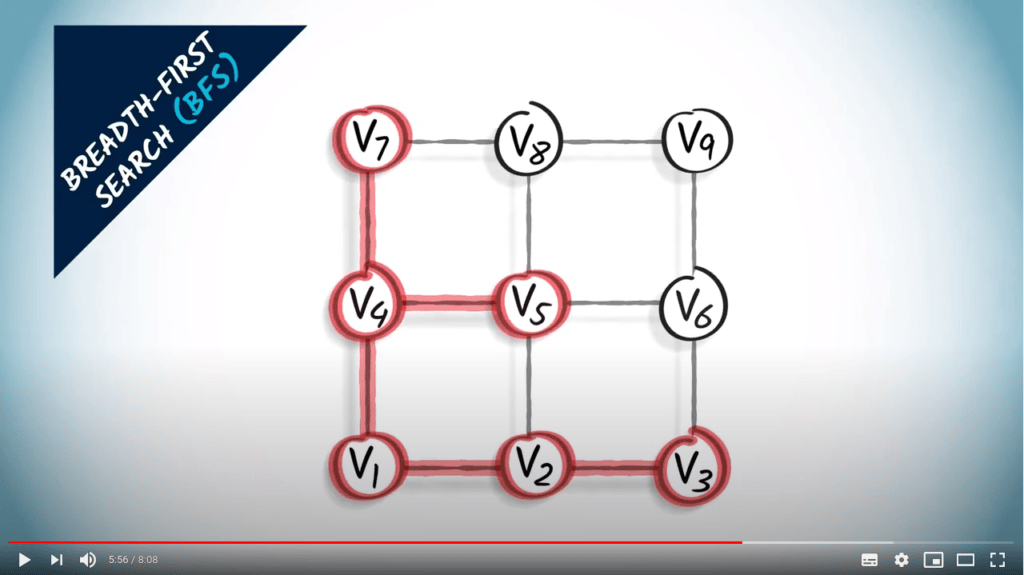
Ensuite, nous explorons tous les sommets à deux sauts de $v_1$. Un sommet à deux sauts de $v_1$ est à un saut d’un sommet qui est lui-même à un saut de $v_1$. Nous regardons donc les voisins de $v_2$ et $v_4$ et les connectons à $v_2$ ou $v_4$. Nous obtenons $v_3$, $v_5$ et $v_7$.

Ensuite, nous explorons les sommets à trois sauts du sommet $v_1$. Nous regardons donc les sommets à deux sauts, qui sont $v_3$, $v_5$ et $v_7$, et leurs voisins non explorés. Nous obtenons $v_8$ et $v_6$.

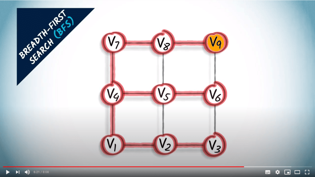
Enfin, le sommet orange est à un saut de $v_8$, qui est à trois sauts du sommet $v_1$. Nous les connectons.

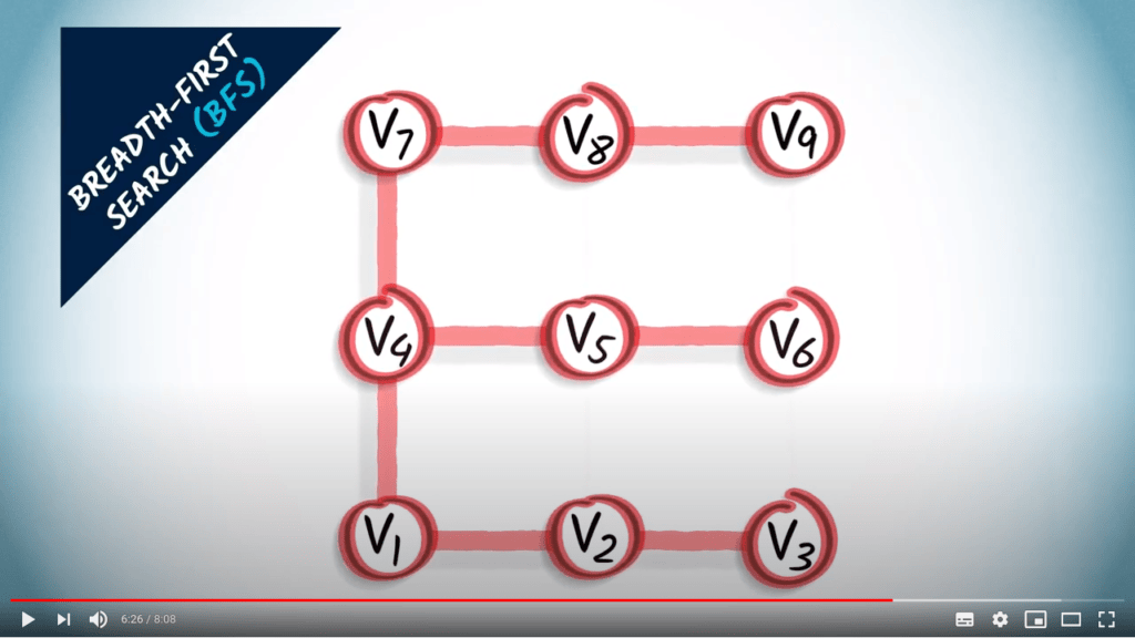
Le graphe résultant en rouge est un arbre couvrant obtenu à partir du BFS, composé exclusivement des plus courts chemins depuis le sommet $v_1$ vers les autres sommets du graphe.

Un BFS est une stratégie prudente dans laquelle nous essayons de maintenir les distances au sommet initial aussi petites que possible pendant l’exploration.

Cela est particulièrement utile lorsque le sommet initial contient des ressources spécifiques dont nous pourrions avoir besoin à tout moment. Cependant, cela nécessite plus d’organisation que son homologue DFS plus simple.

Dans l’exemple précédent, les arbres couvrants obtenus par un BFS et un DFS sont très différents.

Voici un autre exemple utilisant le graphe que nous avons considéré plus tôt dans cette leçon.

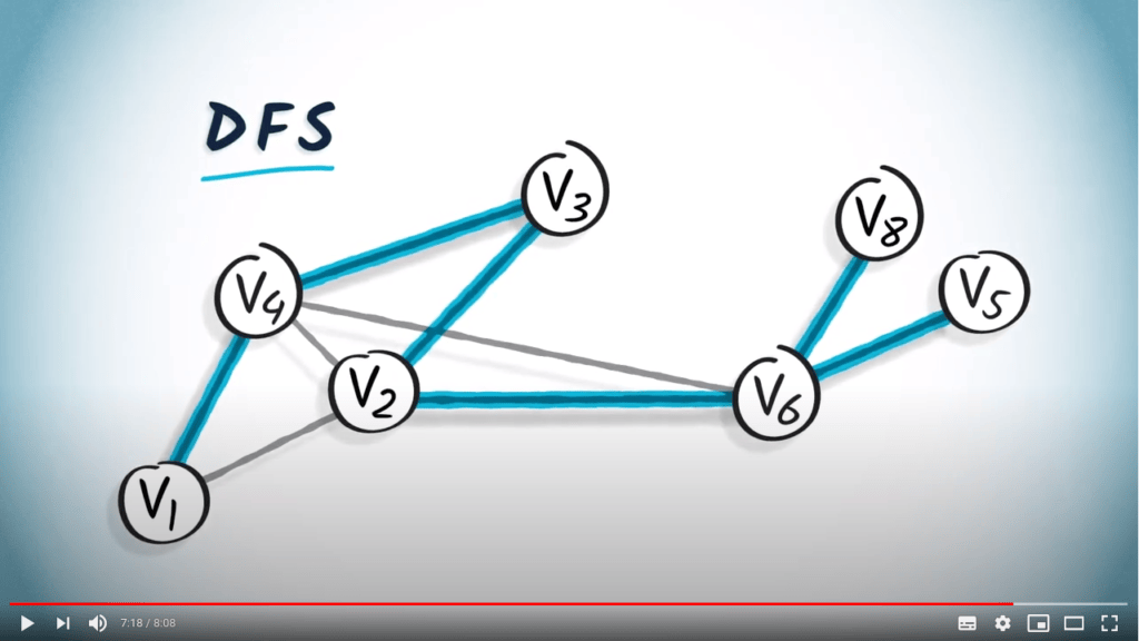
Ceci est un arbre couvrant obtenu à partir d’un DFS en partant de $v_1$.

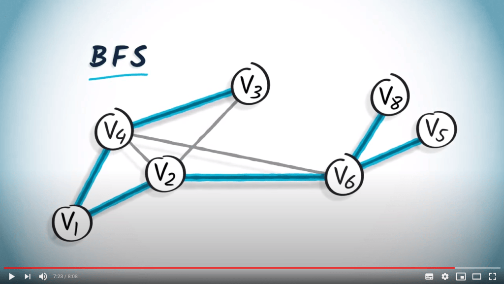
Tandis que ceci est un arbre couvrant obtenu à partir d’un BFS en partant de $v_1$.

Comme un BFS est effectué en augmentant progressivement les sauts depuis $v_1$, un arbre couvrant obtenu à partir d’un BFS fournira toujours le plus court chemin depuis $v_1$ vers tout autre sommet du graphe, à condition que le graphe soit non pondéré. Cela peut être clairement observé dans cet exemple.

Dans la prochaine leçon, nous verrons comment la différence entre un BFS et un DFS est directement liée au type de structure mémoire qui peut être utilisée pour implémenter ces deux algorithmes.