Structures de données & Parcours de graphes
Temps de lecture20 minEn bref
Résumé de l’article
Dans cet article, vous découvrirez certaines structures de données courantes, et comment elles peuvent être utilisées pour façonner le comportement d’un algorithme de parcours. Vous découvrirez les structures LIFO (Last-In First-Out) et FIFO (First-In First-Out), qui définissent respectivement un DFS et un BFS.
Points clés
-
Les structures de données organisent l’information qu’on y stocke selon des règles spécifiques.
-
Certaines structures courantes sont les piles (stacks) et les files (queues).
-
Elles peuvent être utilisées pour façonner le comportement d’un parcours.
-
Le DFS et le BFS peuvent être vus comme un algorithme unique, paramétré avec une pile ou une file.
-
Ces structures de données trouvent des applications dans de nombreuses situations en informatique.
Contenu de l’article
1 — Vidéo
Veuillez consulter la vidéo ci-dessous (en anglais, affichez les sous-titres si besoin). Nous fournissons également une traduction du contenu de la vidéo juste après, si vous préférez.
Important
Certaines “codes” apparaissent dans cette vidéo. Veuillez garder à l’esprit que ce sont des pseudo-codes, c’est-à-dire qu’ils ne sont pas écrits dans un langage de programmation réel. Ça ressemble à du Python, mais ça n’est pas du Python !
Leur but est simplement de décrire les algorithmes sans se soucier des détails de la syntaxe d’un langage de programmation particulier. Vous devrez donc effectuer un peu de travail pour les rendre pleinement fonctionnels en Python si vous souhaitez les utiliser dans vos programmes.
Information
Cliquez ici pour afficher la traduction de la vidéo.

Bonjour, et bienvenue dans cette leçon sur les structures de données pour les parcours.
Dans les leçons précédentes, nous avons examiné les deux principaux algorithmes de parcours de graphes, DFS et BFS, et comment construire et utiliser des tables de routage pour naviguer dans leurs graphes correspondants. Dans cette leçon, nous verrons comment ces algorithmes peuvent être mis en œuvre en pratique, en utilisant des structures de données.
Des structures de données peuvent être utilisées pour gérer les priorités entre les tâches.

Par exemple, imaginez que nous ayons une liste de documents, et que nous devions décider de l’ordre dans lequel nous allons les traiter. Les structures de données peuvent être utilisées pour stocker les documents et gérer la priorité entre eux.
Il y a deux opérations qui peuvent être effectuées lors de l’utilisation d’une structure de données. À savoir, ajouter (ou empiler) un élément, et retirer (ou dépiler) un élément.
Je vais maintenant introduire deux structures de données qui peuvent être utilisées pour gérer les priorités de différentes manières.
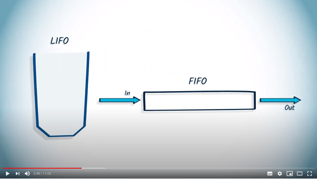
Une pile, connue sous le nom de Last-In First-Out, ou LIFO en abrégé, est une structure de données pour laquelle le dernier élément ajouté dans la pile est le premier à être retiré.

Imaginons une liste de documents que nous devons traiter. Utiliser un LIFO signifie empiler tous les documents, ou les mettre en pile. Vous ne pouvez prendre que le document au sommet de la pile, qui est le dernier ajouté.
Au contraire, une file, connue sous le nom de First-In First-Out, ou FIFO en abrégé, est une structure de données pour laquelle le premier élément ajouté sera le premier à être retiré.

Imaginez cela comme une file d’attente dans un magasin. Les clients sont servis selon le principe du premier arrivé, premier servi.
Une structure de données peut être utilisée pour gérer les priorités avec lesquelles nous examinons les sommets d’un graphe lors d’un parcours de graphe.
Lors de l’exploration d’un sommet, une structure de données peut être utilisée pour stocker les sommets voisins, mais uniquement si ces sommets n’ont pas déjà été explorés.
En répétant ce principe jusqu’à ce que la structure de données soit vide, nous obtenons un DFS si nous choisissons d’utiliser une LIFO, et un BFS lorsque nous utilisons une FIFO.
En effet, en utilisant une LIFO, nous explorons d’abord les derniers sommets ajoutés à la structure de données, et continuons ainsi dans la dernière direction suivie. Cependant, en utilisant une FIFO, nous explorons d’abord les premiers sommets ajoutés, et procédons ainsi par sauts croissants à partir du point de départ.

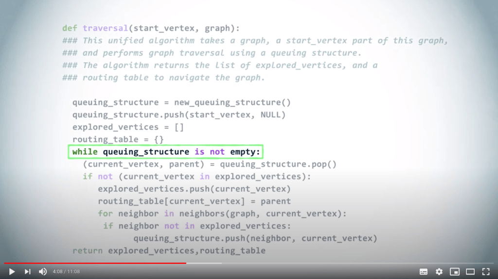
L’algorithme unifié suivant fonctionnera à la fois pour un BFS et un DFS en changeant simplement la structure de données. En d’autres termes, en utilisant une LIFO pour un DFS, et une FIFO pour un BFS.
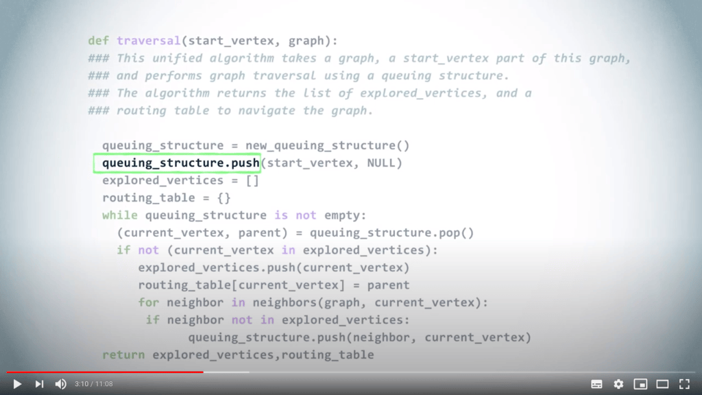
Une fois que nous avons choisi une structure de données, nous commençons par y insérer le sommet de départ. Ici, nous nous intéressons également à la construction de la table de routage, donc, dans la structure de données, nous insérons des couples composés du sommet et de son parent dans l’arbre couvrant correspondant. Comme le sommet de départ n’a pas de parent, nous utilisons NULL à cet endroit.
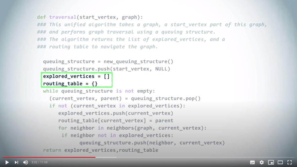
Nous créons également l’ensemble initialement vide des sommets explorés, ainsi que la table de routage initialement vide.
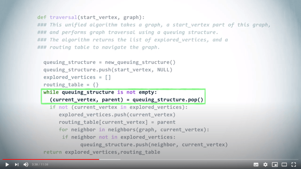
Ensuite, tant que la structure de données n’est pas vide, nous retirons un sommet et son parent.
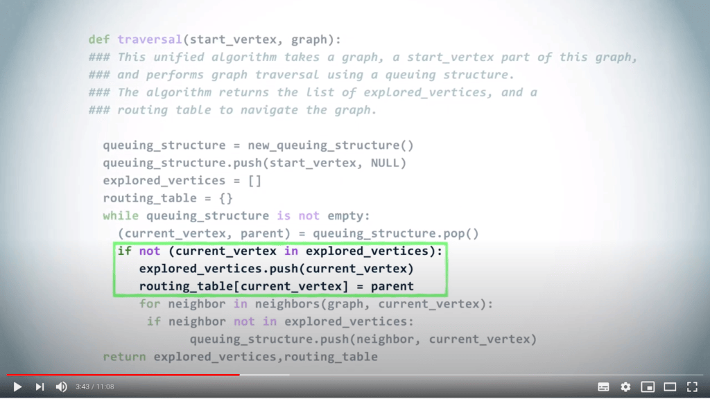
Si ce sommet n’a pas encore été exploré, nous le marquons comme exploré et mettons à jour la table de routage en associant le sommet à son parent.
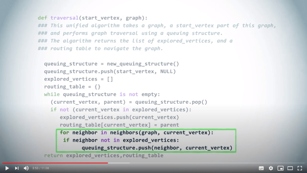
Enfin, nous ajoutons tous les voisins non explorés du sommet à la structure de données, avec le sommet actuel comme parent. Si le sommet que nous avons retiré de la structure de données avait déjà été exploré, nous l’ignorons simplement.
L’algorithme se termine lorsque la structure de données est finalement vide. Selon le choix de la structure de données : une LIFO ou une FIFO, nous obtenons un DFS ou un BFS.
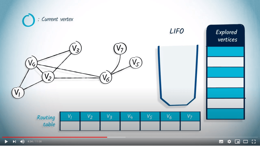
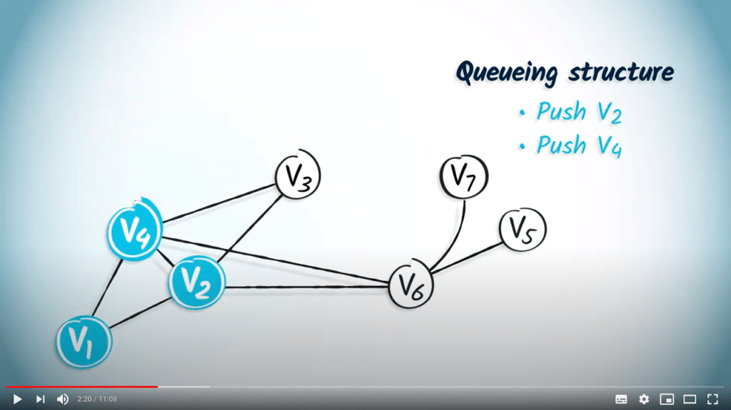
Réalisons un DFS à partir de $v_1$. Nous montrons le contenu de la LIFO pendant que nous parcourons le graphe. La liste des sommets explorés est à droite. Nous affichons également la table de routage.
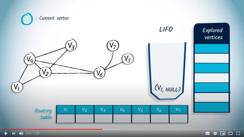
Nous commençons par empiler le sommet de départ $v_1$ dans la LIFO, avec NULL comme parent.
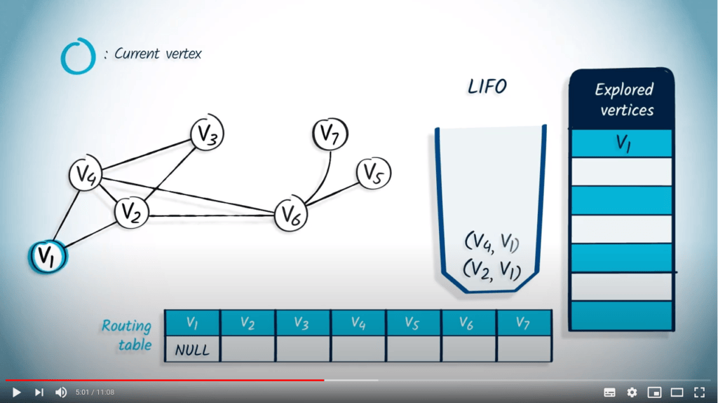
Nous dépilons un sommet et son parent de la LIFO, $v_1$ et NULL. Comme $v_1$ n’est pas dans la liste des sommets explorés, nous le marquons comme exploré et mettons à jour l’entrée correspondante dans la table de routage en la définissant à NULL. Ensuite, nous empilons dans la LIFO tous les voisins de $v_1$ qui ne sont pas dans la liste des sommets explorés, à savoir $v_2$ et $v_4$, avec $v_1$ comme parent.

Nous retirons un élément de la LIFO, qui est $v_4$, avec $v_1$ comme parent, car c’est le dernier élément ajouté. Le sommet $v_4$ n’est pas dans la liste des sommets explorés, donc nous le marquons comme exploré et mettons à jour l’entrée correspondante dans la table de routage en la définissant à $v_1$. Ensuite, nous empilons tous ses voisins non explorés dans la LIFO. Comme $v_1$ a déjà été exploré, nous empilons $v_2$, $v_6$ puis $v_3$ dans la LIFO, avec $v_4$ comme parent.
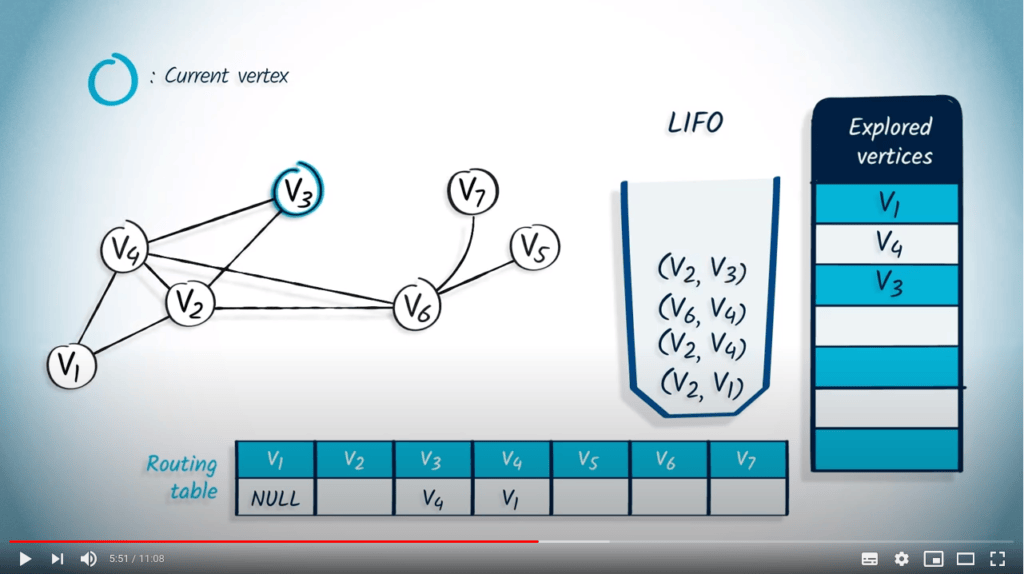
L’élément suivant à être retiré est $v_3$ et son parent $v_4$. Comme $v_3$ n’a pas encore été exploré, nous l’ajoutons à la liste des sommets explorés et mettons à jour la table de routage en conséquence. Parmi les voisins de $v_3$, seul $v_2$ n’a pas été exploré, donc nous empilons $v_2$ dans la LIFO, avec $v_3$ comme parent.
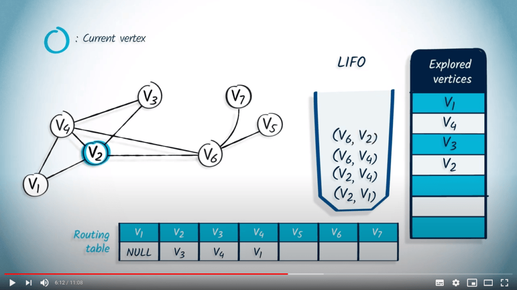
Nous retirons $v_2$ et son parent $v_3$ de la LIFO. Le sommet $v_2$ n’a pas encore été exploré, donc nous le marquons comme exploré et mettons à jour la table de routage en définissant l’entrée correspondante à $v_3$. Parmi les voisins de $v_2$, seul $v_6$ n’a pas été exploré, donc nous empilons $v_6$ avec $v_2$ comme parent dans la LIFO.
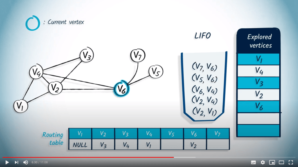
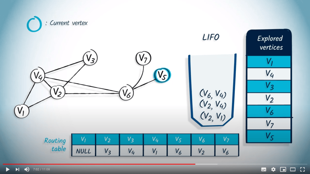
L’élément suivant à être retiré est $v_6$ et son parent $v_2$. Le sommet $v_6$ n’a pas encore été exploré, donc nous le marquons et mettons à jour la table de routage. Les voisins non explorés de $v_6$ sont $v_5$ et $v_7$, donc nous les empilons dans la LIFO avec $v_6$ comme parent.
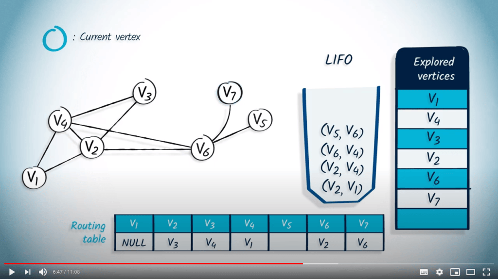
Nous retirons ensuite $v_7$ avec son parent $v_6$. Comme $v_7$ n’a pas encore été exploré, nous le marquons comme exploré et mettons à jour la table de routage. Le seul voisin de $v_7$ est $v_6$, qui a déjà été exploré, donc rien n’est empilé dans la LIFO.
L’élément suivant à être dépilé de la LIFO est $v_5$ et son parent $v_6$. Le sommet $v_5$ n’a pas été exploré, donc nous le marquons comme exploré et mettons à jour la table de routage. Ici encore, le seul voisin de $v_5$ est $v_6$, qui a déjà été exploré, donc rien n’est empilé dans la LIFO.

Ensuite, nous dépilons $v_6$ avec $v_4$ comme parent. Comme $v_6$ a déjà été exploré, rien ne se passe.

Nous retirons $v_2$ avec $v_4$ comme parent, et ici encore, $v_2$ a déjà été exploré, donc rien ne se passe.
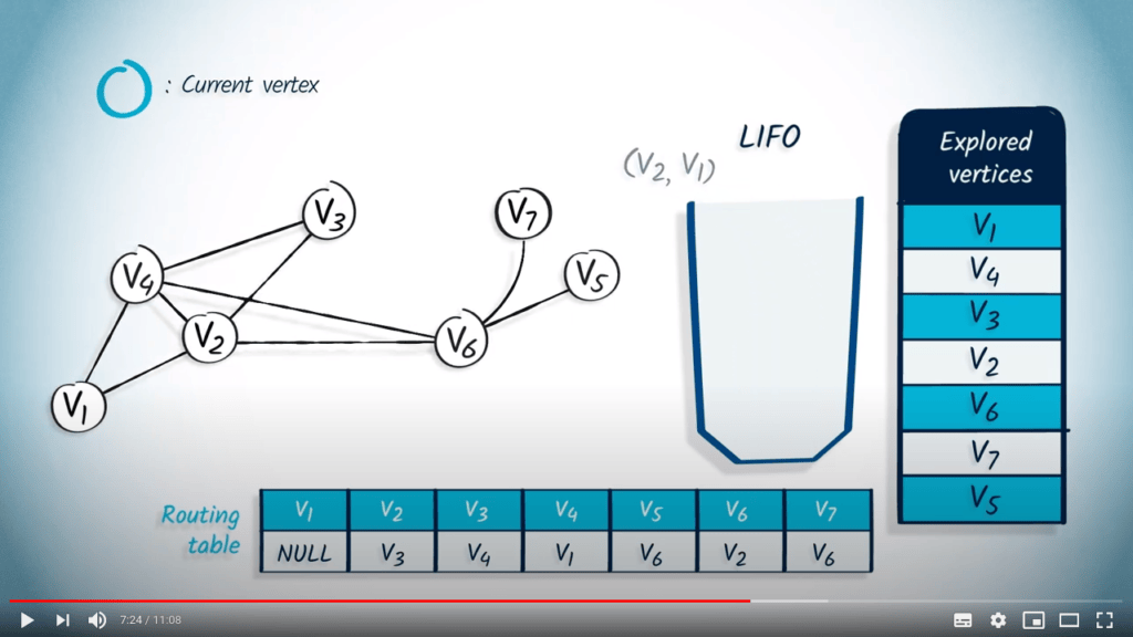
Enfin, $v_2$ avec $v_1$ comme parent est retiré de la LIFO, mais encore une fois, $v_2$ a déjà été exploré, donc rien ne se passe.
La structure de données est maintenant vide, donc l’algorithme termine. Remarquez que le fait d’utiliser une LIFO correspond directement au fait que nous continuons à explorer le graphe jusqu’à ce que la recherche atteigne un sommet sans voisins non explorés, auquel cas nous revenons aux sommets précédemment explorés.
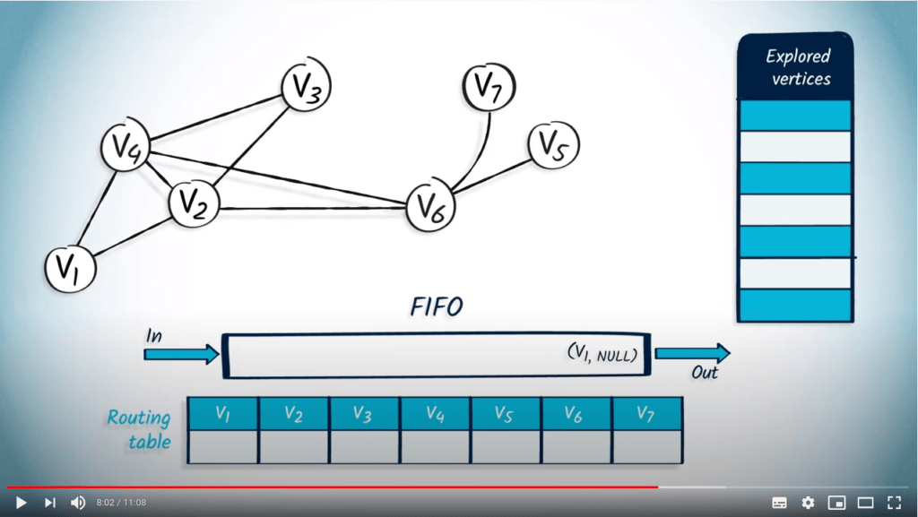
Voyons maintenant comment effectuer un BFS à partir de $v_1$ en utilisant une FIFO. Nous commençons par insérer $v_1$ dans la FIFO, avec NULL comme parent.
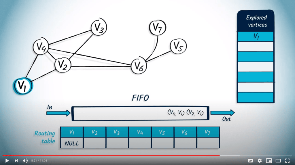
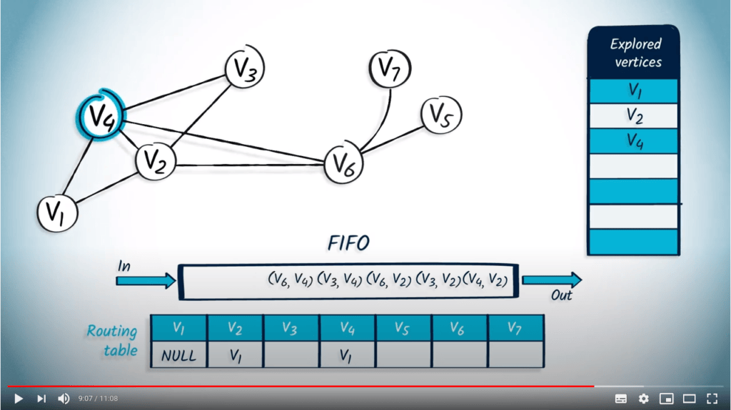
Nous retirons un sommet et son parent de la FIFO, $v_1$ et NULL. Le sommet $v_1$ n’a pas encore été exploré, donc nous le marquons et mettons à jour la table de routage. Ensuite, nous insérons dans la FIFO tous les voisins non explorés de $v_1$, qui sont $v_2$ et $v_4$, avec leur parent $v_1$.

Nous retirons un élément de la FIFO, qui est $v_2$ avec $v_1$ comme parent, car c’est le premier élément qui a été inséré. Le sommet $v_2$ n’a pas encore été exploré, donc nous l’ajoutons à la liste des sommets explorés et mettons à jour la table de routage en conséquence. Nous insérons tous les voisins de $v_2$ qui ne sont pas dans la liste des sommets explorés : $v_4$, $v_3$ et $v_6$, avec $v_2$ comme parent.
L’élément suivant à être retiré de la FIFO est $v_4$ avec $v_1$ comme parent. Comme $v_4$ n’est pas dans la liste des sommets explorés, nous le marquons et mettons à jour la table de routage. Parmi les voisins de $v_4$, seuls $v_3$ et $v_6$ ne sont pas dans la liste des sommets explorés, donc nous les insérons dans la FIFO avec $v_4$ comme parent.
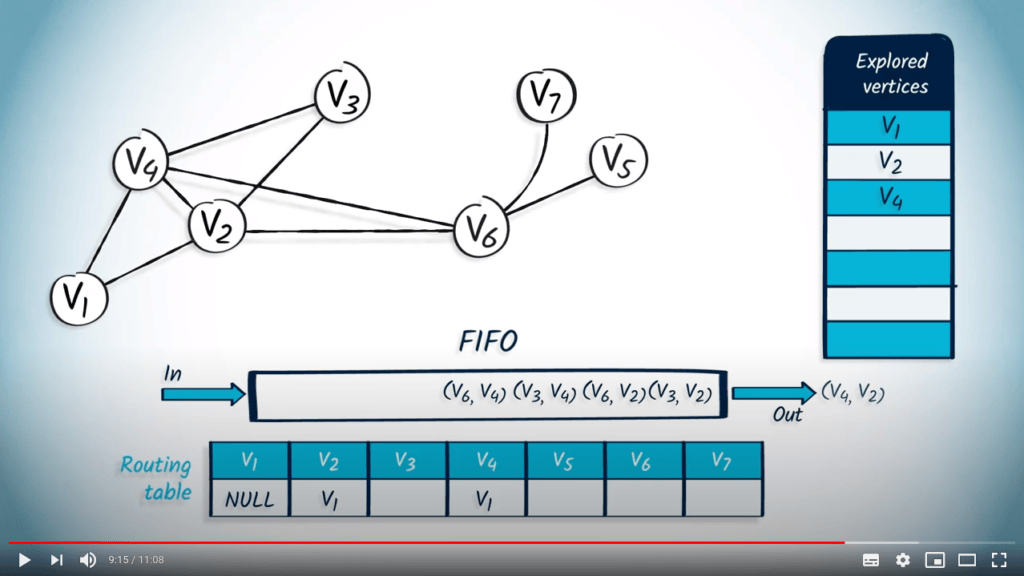
Ensuite, nous retirons l’élément $v_4$ avec $v_2$ comme parent. Le sommet $v_4$ a déjà été exploré, donc nous passons au suivant.
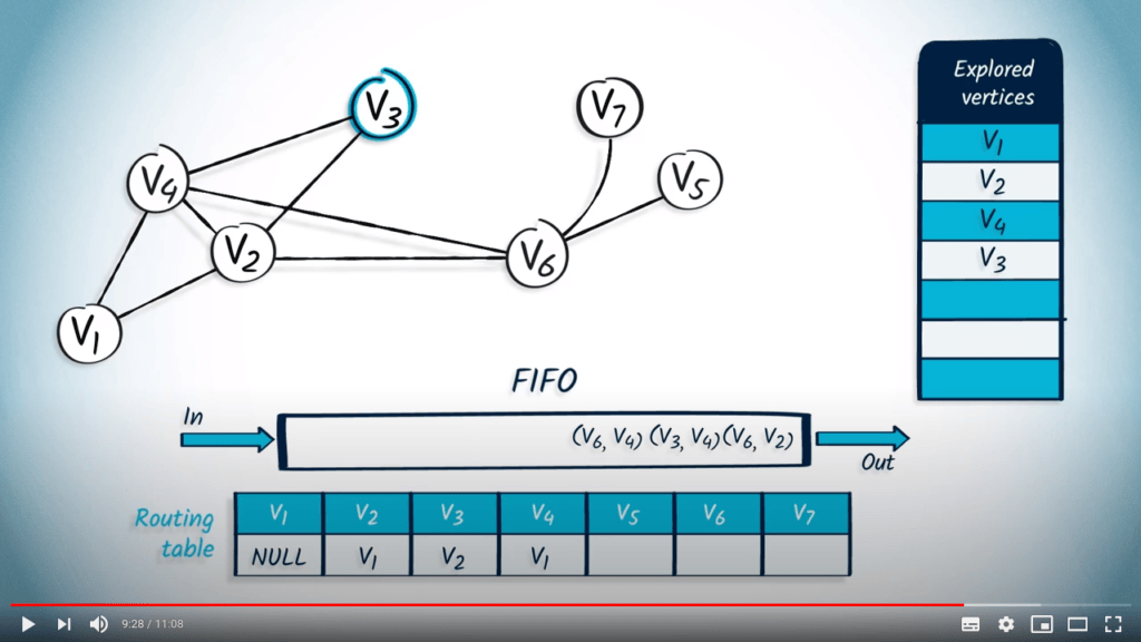
Nous retirons le prochain élément de la FIFO, $v_3$ avec $v_2$ comme parent. Le sommet $v_3$ n’avait pas encore été exploré, donc nous le marquons et mettons à jour la table de routage en conséquence. Tous les voisins de $v_3$ ont été explorés, donc nous continuons.
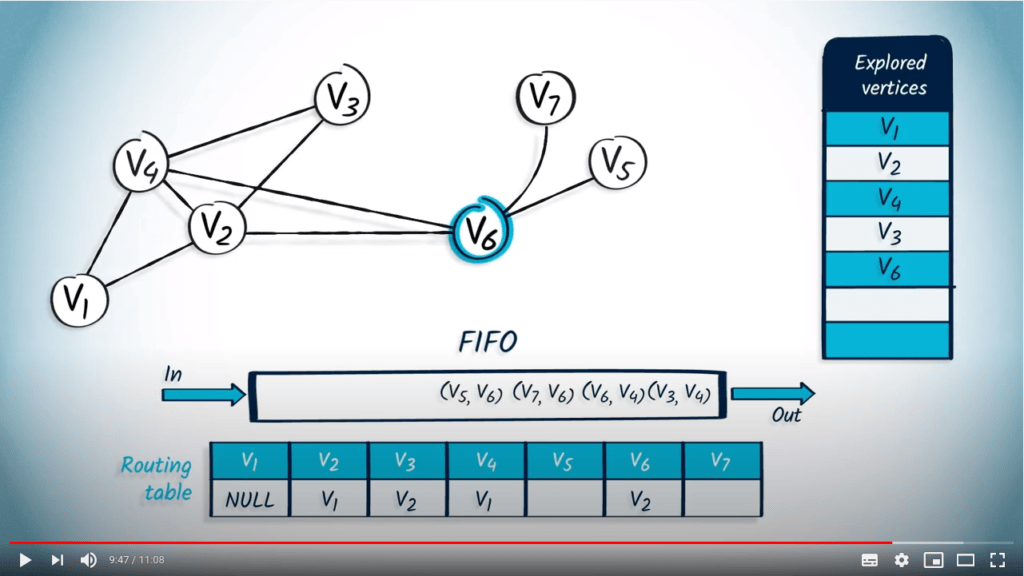
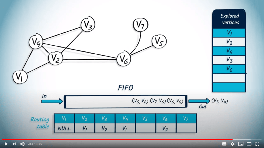
L’élément suivant à être retiré de la FIFO est $v_6$ avec $v_2$ comme parent. Ce sommet n’avait pas encore été exploré, donc nous le marquons et mettons à jour la table de routage. Parmi les voisins de $v_6$, seuls deux voisins ne sont pas explorés : $v_7$ et $v_5$, donc nous les insérons dans la FIFO avec $v_6$ comme parent.
Nous retirons l’élément $v_3$ avec $v_4$ comme parent, mais comme $v_3$ a déjà été exploré, rien ne se passe.
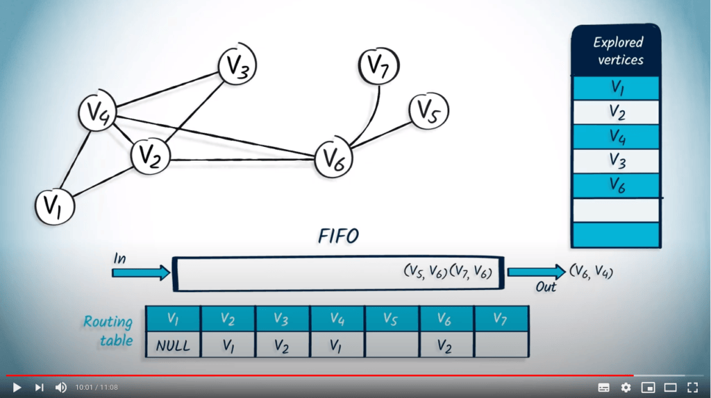
De même, $v_6$ avec $v_4$ est retiré de la FIFO, mais comme $v_6$ a déjà été exploré, nous passons au suivant.
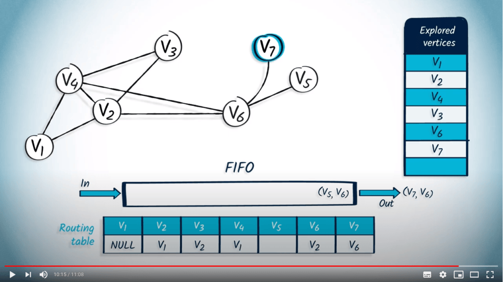
Maintenant, nous retirons de la FIFO l’élément $v_7$ avec $v_6$ comme parent. Le sommet $v_7$ n’avait pas encore été exploré, donc nous le marquons et mettons à jour la table de routage. Le seul voisin de $v_7$ est $v_6$, qui avait déjà été exploré, donc nous continuons.

Enfin, nous retirons $v_5$ avec $v_6$ comme parent de la FIFO. Le sommet $v_5$ n’est pas dans la liste des sommets explorés, donc nous l’ajoutons à cette liste et mettons à jour la table de routage. Ici encore, $v_5$ n’a aucun voisin non exploré.
La structure de données est maintenant vide, donc l’algorithme se termine. Nous avons maintenant parcouru avec succès le graphe en utilisant le BFS.
Ainsi, c’est de cette manière que vous pouvez utiliser les structures de données pour implémenter les algorithmes DFS et BFS.
Merci d’avoir suivi cette leçon ! J’espère que vous avez apprécié apprendre sur les structures de données. C’est la fin des leçons de cette semaine. La semaine prochaine, nous verrons comment traiter les graphes pondérés.
Pour aller plus loin
2 — FIFOs et LIFOs en informatique
Pour illustrer l’importance de ces deux structures de données en informatique, nous présentons deux exemples de situations réelles dans lesquelles elles sont utilisées.
2.1 — Les FIFOs dans les systèmes de communication
Pour que deux personnes communiquent, elles doivent s’envoyer des messages. Et, pour que deux personnes se comprennent, elles doivent s’envoyer des messages dans un ordre logique. Vous comprendrez plus facilement la phrase “L’ordinateur permet à l’homme de faire des erreurs encore plus rapidement que n’importe quelle autre invention, à l’exception peut-être des armes à feu et de la téquila” que “Faire feu et peut-être rapidement n’importe l’ordinateur autre téquila l’exception des à de la armes encore invention permet des erreurs à l’homme de plus que quelle, à”.
Pour les machines, c’est pareil : l’ordre est important et doit être pris en compte. Certains modèles de communication (d’autres sont beaucoup plus complexes) utilisent des files pour cet objectif. Imaginez un modèle dans lequel nous avons un ordinateur $A$ qui écrit des mots dans une file, et un ordinateur $B$ qui les lit. Si l’ordinateur $A$ envoie les mots dans un ordre donné, alors $B$ les lira dans le même ordre (car le premier élément inséré dans une file est aussi le premier à en sortir), et la communication sera possible.
Vous vous demandez peut-être pourquoi passer par une FIFO et ne pas envoyer directement l’information ? L’avantage est que les ordinateurs $A$ et $B$ ne fonctionnent pas nécessairement à la même vitesse (qualité du processeur, carte réseau…). Ainsi, si l’ordinateur $A$ envoie des messages très rapidement à l’ordinateur $B$ (directement), ce dernier en manquera certains. Passer par une file permet de stocker les messages, dans l’ordre, pour éviter ces problèmes de synchronisation.
2.2 — Les LIFOs dans les langages de programmation
Lorsqu’un système d’exploitation exécute un programme, il lui alloue de la mémoire pour qu’il puisse effectuer ses calculs correctement. Cette mémoire est généralement divisée en deux zones : le tas (heap) qui stocke les données, et la pile (stack) qui permet (entre autres) d’appeler des fonctions dans les programmes.
Dans la plupart des langages de programmation, lorsqu’une fonction f(a, b) est appelée à un endroit du code, la séquence (simplifiée) suivante se produit :
- L’adresse de retour est empilée dans la pile.
Cela permettra de revenir juste après l’appel de
fune fois son exécution terminée. - L’argument
aest empilé dans la pile. - L’argument
best empilé dans la pile. - Le processeur est informé de traiter le code de
f. - On dépile un élément de la pile pour obtenir
b. - On dépile un élément de la pile pour obtenir
a. - Le code de
fest exécuté. - Une fois
fterminé, on dépile un élément de la pile pour obtenir l’adresse de retour et revenir à l’endroit oùfa été appelé. - Le processeur est informé de sauter à cette adresse.
Mais pourquoi utiliser une pile au lieu de variables pour transmettre ces informations ?
Eh bien, le processeur ne connaît pas les détails de f !
Il est possible que f utilise une autre fonction g, par exemple.
Si des variables étaient utilisées, l’adresse de retour de f serait écrasée par l’adresse de retour de g, et lorsque g serait terminé, il serait impossible de revenir au moment de l’appel de f.
Et pourquoi pas une FIFO alors ?
Ici encore, le problème se pose si f appelle une fonction g.
Comme l’adresse de retour de f est placée avant celle de g dans la file, lorsqu’il sera nécessaire de revenir de l’appel à g, le processeur obtiendra à la place l’adresse de retour de f (la plus ancienne dans la file) !
Nous n’exécuterons donc jamais le code de f situé après l’appel à g.
Pour aller encore plus loin
- Théorie des files d’attente.
Fournit des résultats supplémentaires sur les files (temps moyen avant d’être extrait, etc.) et a de nombreuses applications.