Representer les graphes
Temps de lecture5 minEn bref
Résumé de l’article
Dans cet article, vous découvrirez des solutions pour représenter des graphes en mémoire dans un ordinateur. Après la vidéo, nous vous présenterons la structure de graphe que vous manipulerez dans le projet PyRat.
À retenir
-
La matrice d’adjacence d’un graphe peut être représentée en mémoire à l’aide d’un tableau.
-
Les listes et les dictionnaires sont également des solutions pour représenter un graphe en mémoire.
-
Chaque représentation a ses propres avantages et inconvénients.
-
Dans PyRat, la représentation d’un graphe est abstraite dans un objet.
Contenu de l’article
1 — Vidéo
Veuillez consulter la vidéo ci-dessous (en anglais, affichez les sous-titres si besoin). Nous fournissons également une traduction du contenu de la vidéo juste après, si vous préférez.
Information
Cliquez ici pour afficher la traduction de la vidéo.

Bonjour tout le monde ! Dans cette leçon, nous allons parler de la manière de choisir des structures de données pour représenter des graphes.

Comme vous le savez sûrement, la mémoire informatique est organisée en emplacements où les données sont stockées.
Accéder aux données nécessite donc de connaître l’emplacement (ou l’adresse) où elles ont été stockées.

De la même manière qu’il est plus facile de trouver une maison par son adresse plutôt que par sa description, ou un livre de bibliothèque par son numéro d’appel, il est plus facile de trouver des données lorsque vous connaissez leur adresse spécifique.
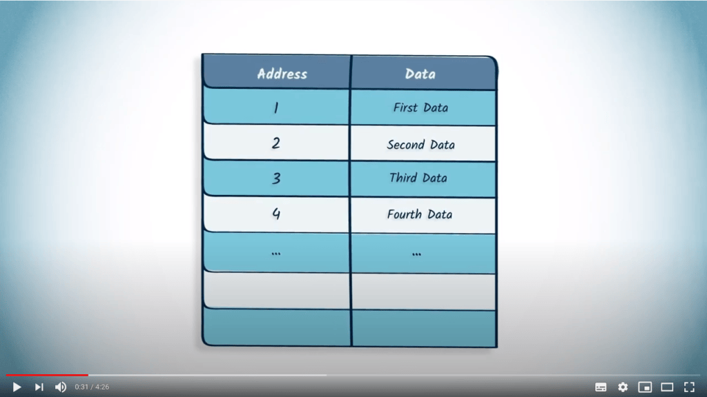
Imaginons que nous souhaitons stocker la matrice d’adjacence d’un graphe. Une façon de stocker des données en mémoire est d’utiliser un tableau. Les tableaux sont des structures de données adjacentes utilisées pour représenter des séquences de données, où chaque élément utilise la même taille en mémoire.
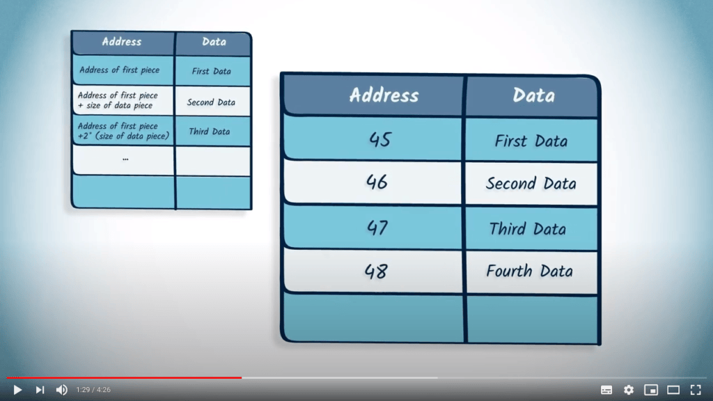
Ainsi, si vous connaissez l’adresse du premier élément, l’adresse de tout autre élément peut facilement être calculée. Par exemple, si l’adresse du premier élément est 45, et si chaque élément utilise une adresse, alors l’adresse du quatrième élément est 48.
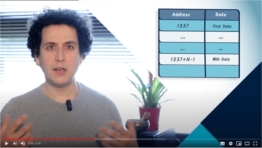
Cela signifie que vous pouvez accéder rapidement au $n^{ième}$ élément d’un tableau. En revanche, accéder au $n^{ième}$ élément non nul peut prendre du temps, car toutes les cellules doivent être vérifiées une par une pour voir si elles contiennent un zéro ou non.
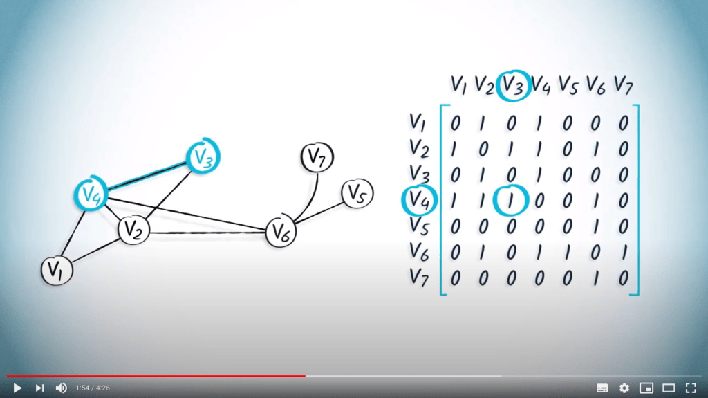
En termes de matrices d’adjacence de graphes, les tableaux sont efficaces pour vérifier si deux sommets $u$ et $v$ sont connectés par une arête.
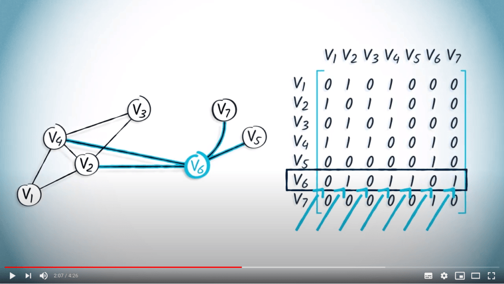
En revanche, ils ne sont pas aussi efficaces si vous voulez récupérer tous les voisins de $u$, car vous devez tester chaque sommet $v$ un par un.
Une autre structure de données courante est une liste. Les listes ne sont pas adjacentes en mémoire, et pour trouver un élément, vous devez d’abord trouver tous les éléments précédents.

Le principe des listes est que chaque adresse contient non seulement des données, mais aussi l’adresse de l’élément suivant à rechercher.
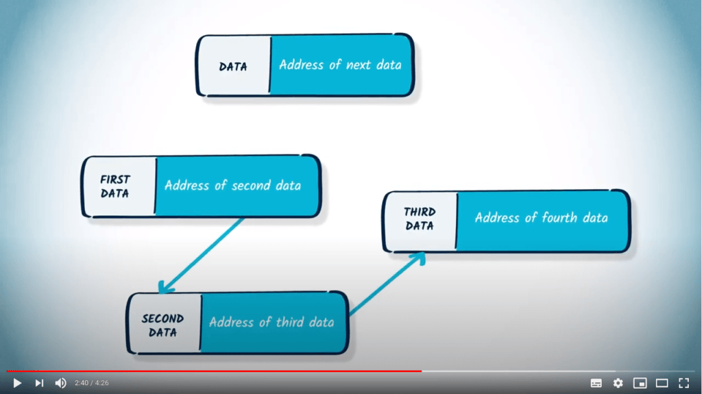
Ainsi, si vous voulez accéder au troisième élément d’une liste, vous devez d’abord accéder au premier, regarder l’adresse du deuxième, puis regarder le deuxième pour trouver l’adresse du troisième.
Accéder au $n^{ième}$ élément d’une liste peut prendre du temps. Cependant, il est possible de surmonter ce processus chronophage en ne stockant que les éléments d’intérêt, ce qui réduit considérablement l’utilisation de la mémoire par rapport à un tableau.
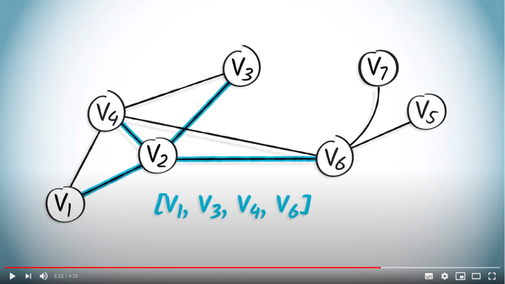
En termes de graphes, les listes peuvent être utilisées pour stocker uniquement des informations sur les voisins des sommets, par exemple, puisque les non-voisins sont souvent non pertinents. Si chaque sommet n’a que quelques voisins, représenter uniquement les voisins avec des listes peut permettre d’économiser considérablement de la mémoire. En revanche, vérifier si $u$ et $v$ sont connectés par une arête peut nécessiter de parcourir toute la liste des voisins de $u$.
Une dernière structure de données est le dictionnaire. Les dictionnaires sont des structures élaborées qui visent à combiner les avantages des tableaux et des listes. En particulier, un accès rapide et une utilisation efficace de la mémoire.
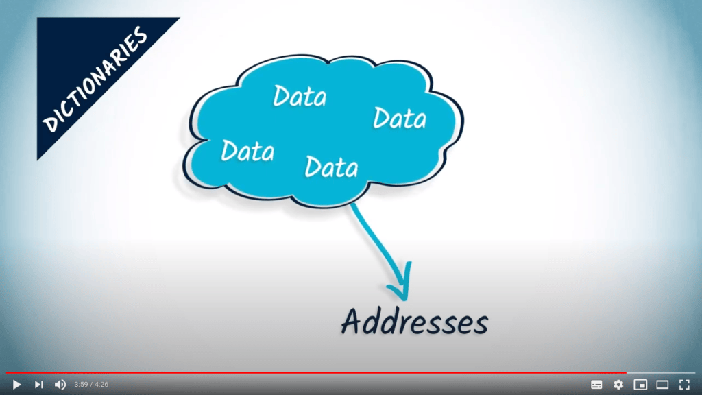
Les dictionnaires utilisent des fonctions de hachage, qui sont essentiellement des mécanismes pour transformer des contenus en adresses. C’est le choix optimal pour le prototypage, car il permet aux programmeurs de bénéficier à la fois de la rapidité d’accès et d’une faible utilisation de la mémoire.
En règle générale, les dictionnaires devraient toujours être utilisés si vous ne savez pas exactement ce que vous faites.
Merci pour votre attention ! C’est tout pour les structures de mémoire, et je vous retrouverai très bientôt pour parler des bonnes pratiques de programmation. Au revoir !
2 — La représentation d’un graphe dans PyRat
Dans le logiciel PyRat, le graphe est encapsulé dans un objet, i.e., une structure complexe qui vous fournit une interface pratique pour le manipuler. En d’autres termes, vous n’avez pas un accès direct à la matrice d’adjacence, à la liste ou au dictionnaire qui stocke le graphe en mémoire. À la place, vous avez accès à de nombreux attributs et méthodes qui vous permettent de manipuler le graphe sans entrer dans les détails de son implémentation.
Plus précisément, soit g une instance de la classe Graph de PyRat.
Vous pouvez utiliser les fonctions décrites dans la documentation de la classe Game.
Information
En pratique, un labyrinthe PyRat est une instance de la classe Maze, qui hérite de Graph.
Ainsi, il possède quelques attributs supplémentaires (e.g., une width et une height en nombre de cases) et des méthodes supplémentaires (e.g., coords_difference(v1, v2) pour obtenir la différence selon les axes de largeur et de hauteur, i_exists(v) pour vérifier qu’une case existe dans le labyrinthe).
Consultez la documentation de la classe Maze pour plus d’informations !
Vous voyez, à aucun moment vous n’avez besoin de connaître la structure sous-jacente pour utiliser le graphe dans votre projet. C’est très pratique si le développeur de PyRat décide un jour de modifier cette structure pour une raison quelconque. En effet, tant que l’interface reste inchangée, le code des utilisateurs continuera de fonctionner.
Information
Il existe de nombreuses bibliothèques en ligne qui fournissent de telles interfaces pour utiliser des graphes. Quel que soit le langage que vous utilisez, il est toujours judicieux de vérifier les implémentations existantes avant de réimplémenter une structure à partir de zéro !
Pour aller plus loin
3 — Plus de détails sur la solution basée sur les listes
Nous avons vu précédemment qu’une matrice d’adjacence est un objet pratique pour représenter un graphe en mémoire.
Cependant, dans la plupart des cas, les graphes sont des objets creux, i.e., le nombre d’arêtes existantes est faible par rapport au nombre d’arêtes d’un graphe complet. Une conséquence directe est que la plupart des entrées de la matrice d’adjacence sont des 0. Étant donné que le nombre d’éléments dans une matrice d’adjacence est égal au carré de l’ordre du graphe, cela peut rapidement entraîner une utilisation importante de l’espace mémoire.
Une solution possible pour contourner ce problème est d’utiliser une structure de données différente : une liste de listes. Appelons un tel objet $L = (l_1, \dots, l_n)$, avec $l_1, \dots, l_n$ étant des listes. Dans cette structure, $l_i$ $(i \in [1, n])$ représentera les arêtes accessibles depuis le sommet $i$.
À titre d’exemple, considérons la matrice d’adjacence suivante : $${\bf A} = \begin{pmatrix} 0 & 1 & 0 & 1 & 0 & 0 & 0 \\ 1 & 0 & 1 & 1 & 0 & 1 & 0 \\ 0 & 1 & 0 & 1 & 0 & 0 & 0 \\ 1 & 1 & 1 & 0 & 0 & 1 & 0 \\ 0 & 0 & 0 & 0 & 0 & 1 & 0 \\ 0 & 1 & 0 & 1 & 1 & 0 & 1 \\ 0 & 0 & 0 & 0 & 0 & 1 & 0 \end{pmatrix}$$
En supposant que les sommets soient étiquetés de 1 à $n$, cette matrice est équivalente à la liste $L = ( (2, 4) , (1, 3, 4, 6), (2, 4), (1, 2, 3, 6), (6), (2, 4, 5, 7), (6) )$.
On peut rapidement remarquer que le nombre de nombres stockés est passé de $n^2$ = 49 à 18.
Bien que cette solution permette d’économiser de l’espace mémoire, elle présente certaines limitations :
-
Vérifier l’existence d’une arête ${i, j}$ nécessite de parcourir tous les éléments de la liste $l_i$ pour vérifier si $j$ en fait partie. Cela peut prendre du temps si $i$ a de nombreux voisins. En comparaison, effectuer la même vérification avec une matrice d’adjacence ${\bf A}$ ne nécessite qu’une seule opération, car il suffit de vérifier que ${\bf A}[i, j] \neq 0$.
-
Elle est moins facile à étendre aux graphes pondérés. Dans le cas des matrices d’adjacence, les entrées représentent le poids associé à l’arête. Ici, les entrées sont les indices des éléments non nuls, qui ne peuvent pas être modifiés sans créer ou supprimer des arêtes. Une solution possible consiste à remplacer les listes d’indices $l_i = (j, k, \dots)$ par des listes de couples $l_i = ( (j, w_j), (k, w_k), \dots )$, où $w_j$ est le poids de l’arête ${i, j}$.
Pour aller encore plus loin
-
Understanding the Efficiency of GPU Algorithms for Matrix-Matrix Multiplication.
Un article de recherche illustrant l’une des principales raisons pour lesquelles les matrices sont fréquemment utilisées.
-
Graph Processing on FPGAs: Taxonomy, Survey, Challenges.
Un article de recherche illustrant l’utilisation de matériel spécifique (ici, FPGA) pour traiter de grands graphes.