Tables de routage
Temps de lecture10 minEn bref
Résumé de l’article
Dans cet article, vous apprendrez à stocker le résultat d’un parcours dans une structure de données appelée table de routage. Ensuite, vous apprendrez à utiliser cette structure pour retrouver le chemin trouvé par le parcours jusqu’à un sommet donné. Après la vidéo, nous établirons un lien entre les tables de routage et certaines structures de données que vous avez déjà vues.
À retenir
-
Les tables de routage permettent de stocker le résultat d’un parcours de graphe en mémoire.
-
Elles peuvent ensuite être utilisées pour analyser le parcours effectué, par exemple pour trouver un chemin.
-
Elles peuvent être implémentées à l’aide d’une liste ou d’un dictionnaire.
Contenu de l’article
1 — Vidéo
Veuillez consulter la vidéo ci-dessous (en anglais, affichez les sous-titres si besoin). Nous fournissons également une traduction du contenu de la vidéo juste après, si vous préférez.
Information
Cliquez ici pour afficher la traduction de la vidéo.
Bonjour tout le monde ! Dans la leçon d’aujourd’hui, nous allons voir comment construire des tables de routage pour naviguer dans un graphe, en utilisant les arbres couvrants obtenus à partir d’algorithmes de parcours de graphe, tels que le BFS ou le DFS. Ces tables de routage aideront l’intelligence artificielle que vous développerez dans ce cours à se déplacer entre deux positions dans le labyrinthe.
Dans la leçon précédente, vous avez appris à construire des arbres couvrants. Une fois que nous avons un tel arbre couvrant, nous avons besoin d’un algorithme de routage pour pouvoir naviguer entre n’importe quels deux sommets du graphe.
Le routage d’un point de départ à une destination est interprété à l’envers. Nous savons déjà quel est le point de départ, donc nous devons commencer par la destination pour trouver un chemin. Ainsi, un algorithme de routage fournit un chemin de la destination au point de départ.
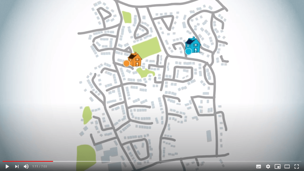
Tracer un chemin à l’envers est plus intuitif qu’il n’y paraît. Imaginez que vous, le cercle bleu sur la carte, devez conduire jusqu’à la maison d’un ami, qui est le cercle orange sur la carte.
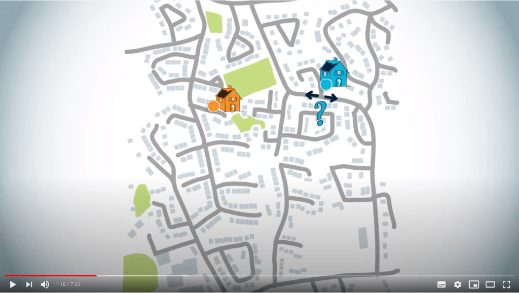
Vous pourriez commencer par décider si vous devez tourner à gauche ou à droite à la prochaine intersection.
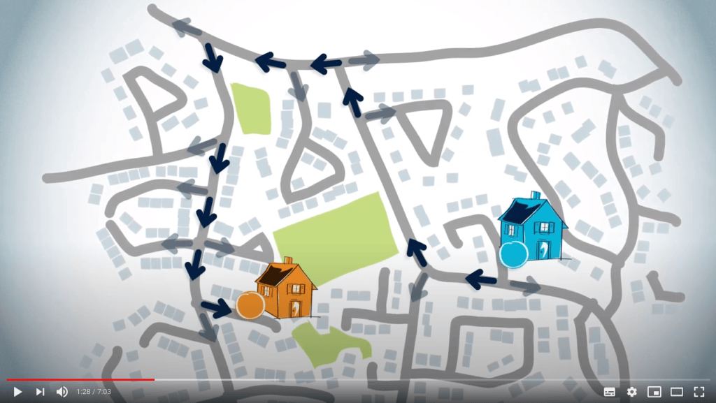
Ensuite, à chaque intersection que vous rencontrez, identifiez quelle route peut être empruntée ensuite, jusqu’à ce que vous atteigniez enfin la maison de votre ami.
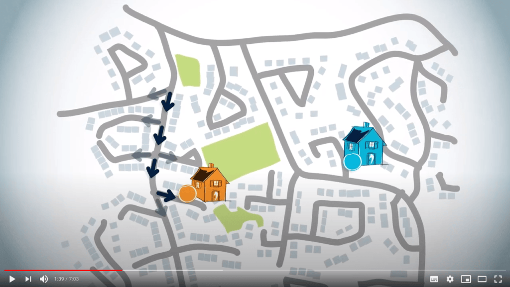
Ou, vous pourriez réfléchir au meilleur itinéraire à l’envers, en identifiant d’abord sur quelle rue se trouve la maison de votre ami. Ensuite, quelle autre route accède à cette rue, etc.
Jusqu’à savoir si vous devez tourner à gauche ou à droite à la prochaine intersection.
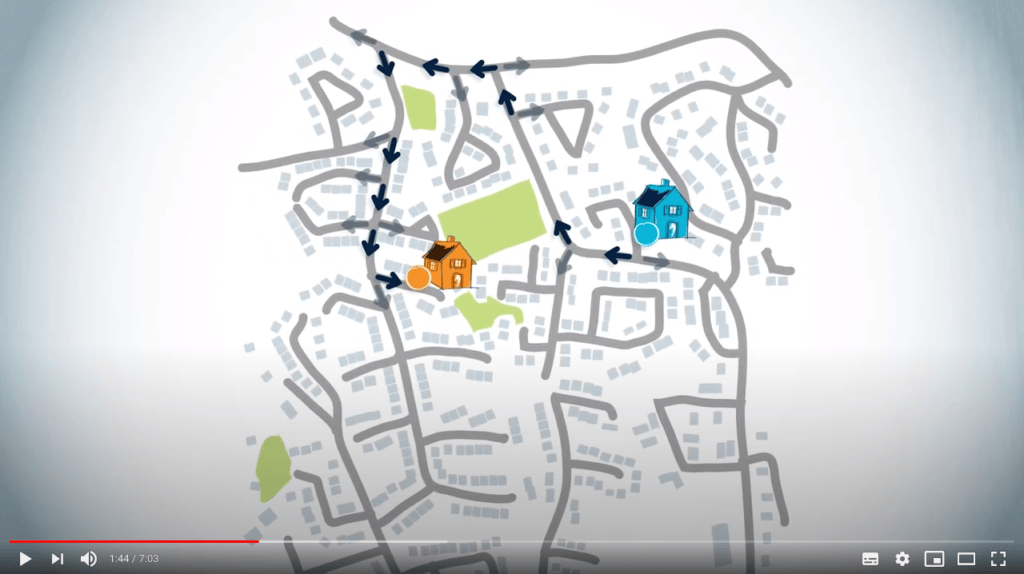
Cette seconde façon de penser est celle utilisée par l’algorithme de routage.
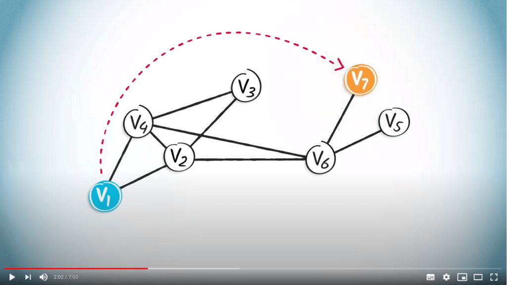
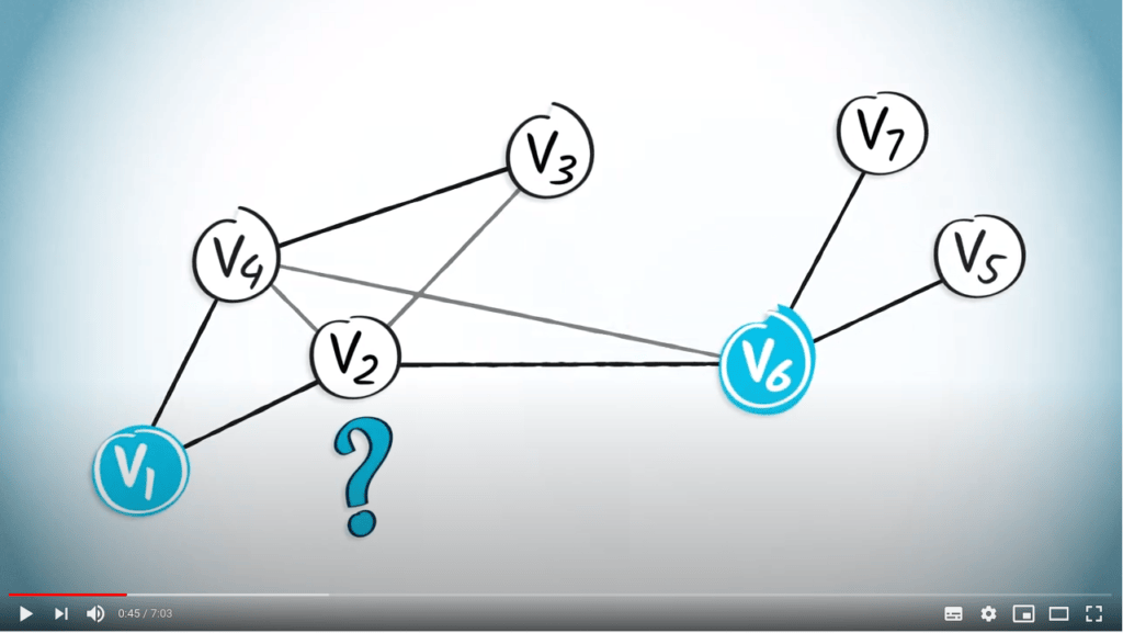
Pour mieux comprendre cela, regardons un exemple que nous avons déjà vu dans la leçon précédente avec Vincent. Considérons le chemin entre $v_1$ et $v_7$.
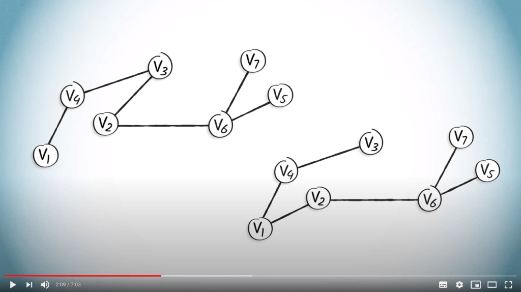
Nous pouvons voir l’arbre couvrant obtenu en utilisant un DFS à gauche, et l’arbre couvrant obtenu en utilisant un BFS à droite.
Le routage de $v_1$ à tout autre sommet peut être facile lorsque nous utilisons des arbres. Mais pour ce faire, nous avons d’abord besoin de quelques définitions supplémentaires.
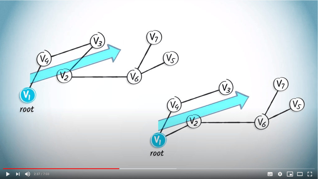
Un arbre enraciné est un arbre dans lequel nous désignons un sommet particulier comme racine, également parfois appelée origine. Dans ce cas, nous considérerons $v_1$ comme la racine, car c’est notre position de départ. Par conséquent, les arêtes de cet arbre enraciné ont une orientation naturelle s’éloignant de la racine.
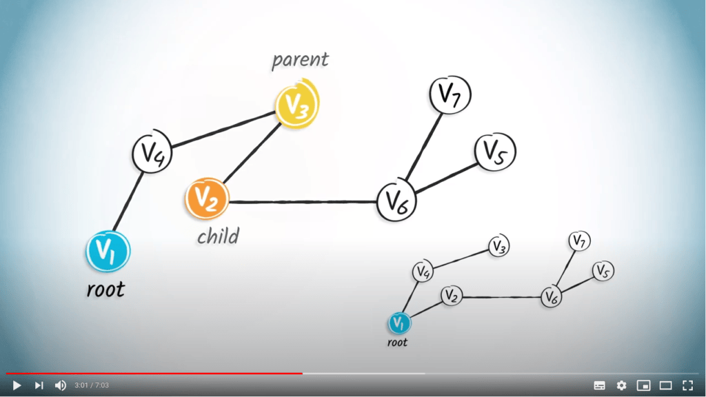
Dans un arbre enraciné, le parent d’un sommet est le sommet qui lui est connecté sur le chemin depuis la racine. Par exemple, le parent de $v_2$ est $v_3$ dans l’arbre de gauche. Chaque sommet, sauf la racine, a un seul parent. Un enfant d’un sommet $v$ est un sommet dont $v$ est le parent. Ainsi, $v_2$ est l’enfant de $v_3$ dans l’arbre de gauche.
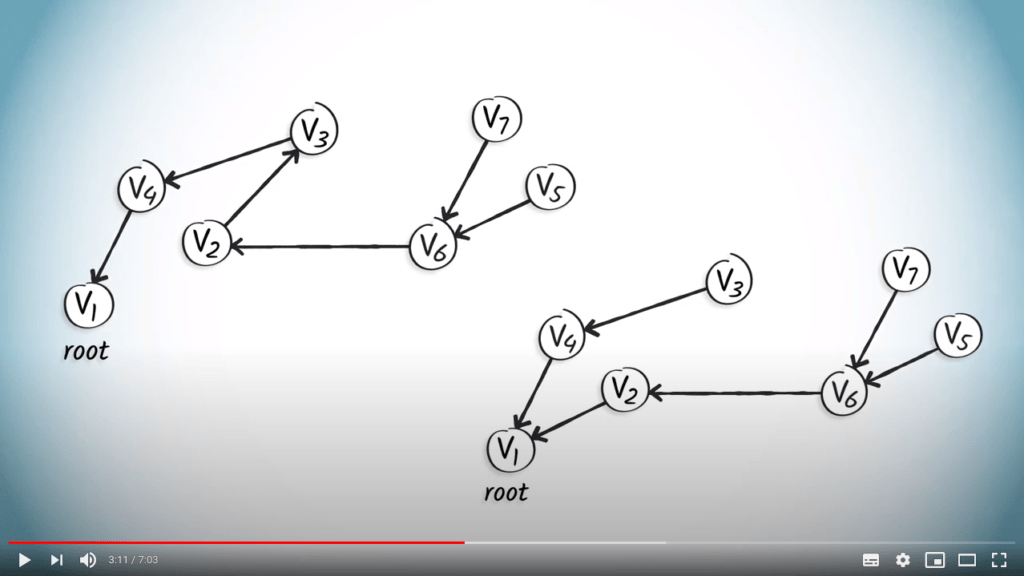
Si nous appliquons ces concepts à l’ensemble des arbres, nous obtenons les arbres enracinés suivants, où l’orientation des arêtes indique les parents des sommets. Par exemple, dans les deux graphes, $v_1$ n’a pas de parent, le parent de $v_4$ est $v_1$, et les enfants de $v_6$ sont $v_7$ et $v_5$.
Nous pouvons maintenant construire des tables de routage en considérant le parent de chaque sommet dans le chemin depuis $v_1$. Les tables de routage sont des structures de données utiles qui permettent de reconstruire un chemin. Comme mentionné précédemment, le routage est considéré à l’envers, de la destination jusqu’à la position de départ.
Une table de routage comporte une seule ligne et autant de colonnes qu’il y a de sommets dans le graphe. Chaque colonne correspond à un sommet, et la valeur associée dans la table est son parent dans l’arbre couvrant enraciné en $v_1$.
Voyons maintenant comment cette table est construite étape par étape à l’aide d’un arbre couvrant.
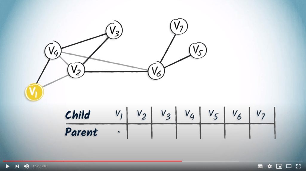
Commençons par un arbre obtenu à partir d’un DFS. Nous partons d’une table vide. Le sommet $v_1$ est la racine, donc il n’a pas de parent. Nous notons simplement un point dans la colonne de $v_1$.
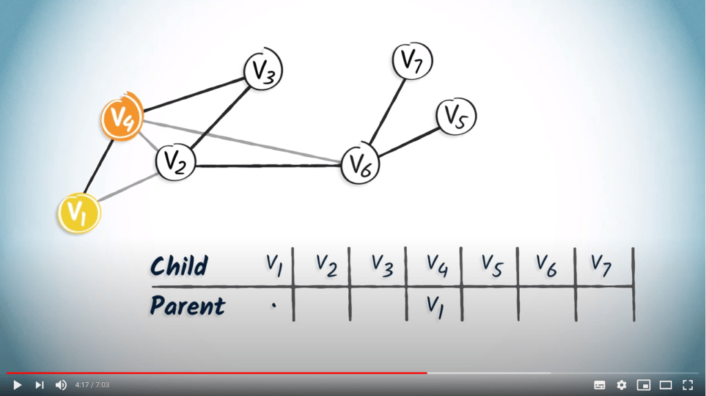
Le sommet $v_1$ n’a qu’un seul enfant, $v_4$. Nous ajoutons donc $v_1$ dans la colonne correspondant à $v_4$.
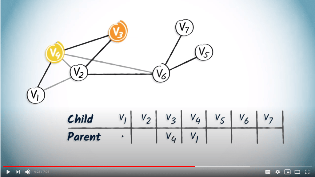
Le sommet $v_4$ n’a qu’un seul enfant, $v_3$. Nous ajoutons donc $v_4$ dans la colonne de $v_3$.
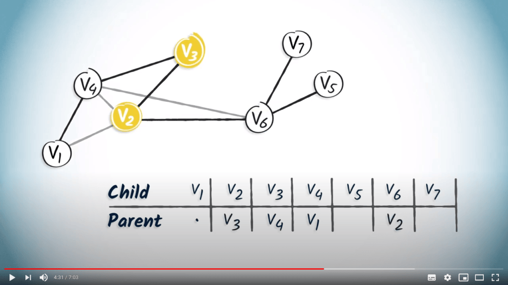
Appliquons maintenant le même principe aux sommets $v_2$ et $v_6$, qui sont les seuls enfants de $v_3$ et $v_2$, respectivement.
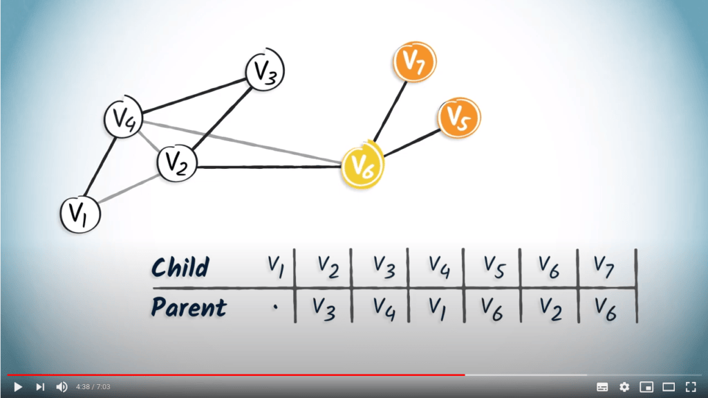
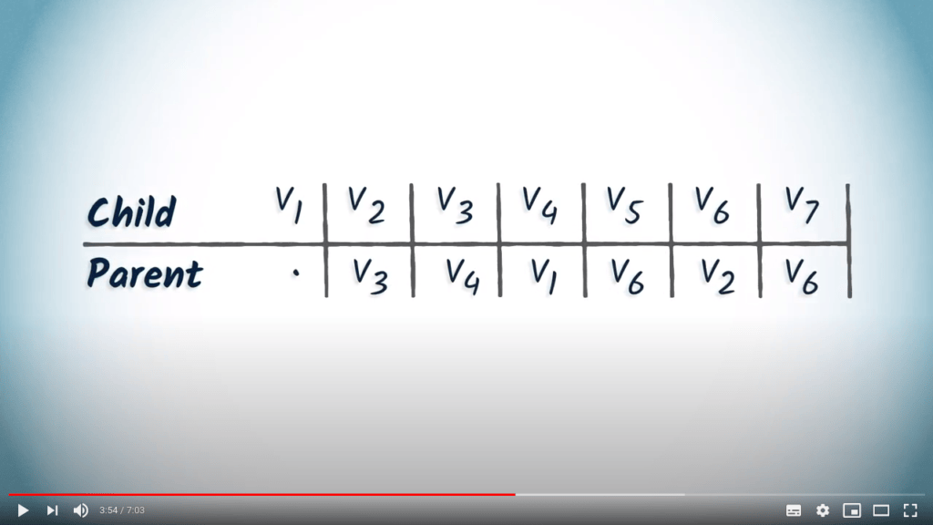
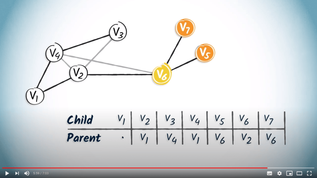
Enfin, $v_6$ a deux enfants, $v_7$ et $v_5$. Ajoutons donc $v_6$ dans les colonnes correspondant à $v_5$ et $v_7$. Voilà, la table de routage est complète.
Pour lire cette table, commencez simplement par la destination souhaitée et lisez l’entrée correspondante, qui fait référence au parent du sommet de destination.
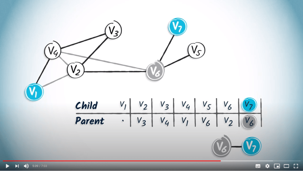
Par exemple, si nous cherchons le chemin de $v_1$ à $v_7$, nous lisons d’abord l’entrée correspondant à $v_7$, qui est $v_6$. Par définition, le parent de la destination correspond à son tour au sommet précédent dans le chemin de $v_1$ à la destination.
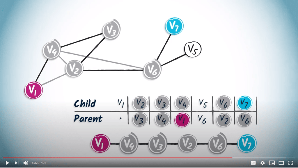
En lisant les entrées correspondant à chaque prédécesseur, vous atteindrez finalement la position de départ $v_1$. Dans notre exemple, l’étape suivante consiste à identifier l’entrée correspondant à $v_6$, qui est $v_2$. En continuant ainsi, nous obtenons le chemin $(v_7, v_6, v_2, v_3, v_4, v_1)$.
En guise de second exemple, construisons également la table de routage à partir de l’arbre couvrant obtenu par un BFS.
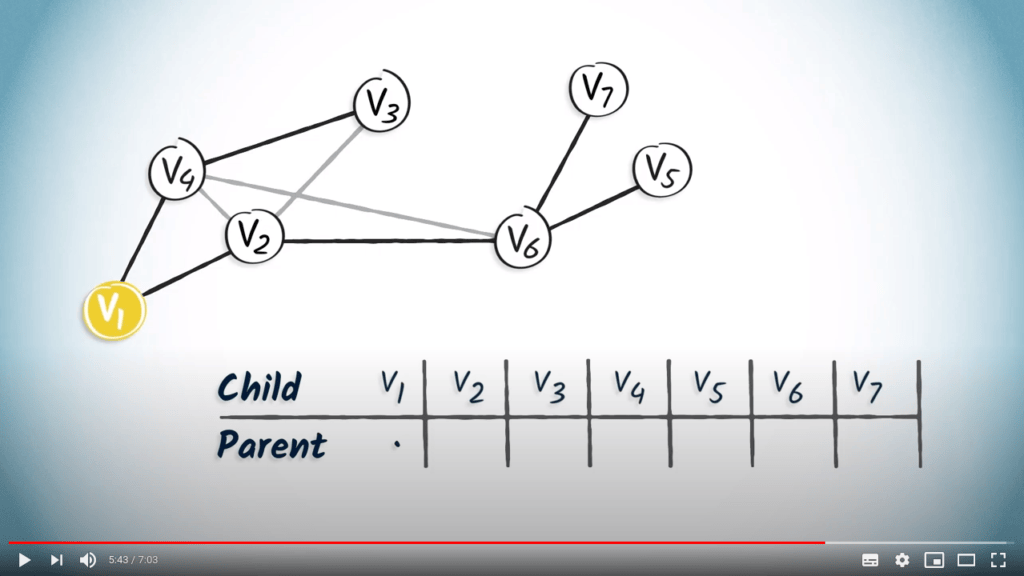
Voici l’arbre couvrant. Encore une fois, nous partons d’une table vide.
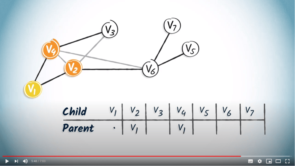
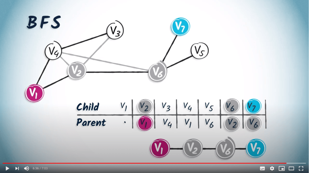
Le sommet $v_1$ a deux enfants, les sommets $v_4$ et $v_2$. Nous ajoutons donc $v_1$ dans les colonnes correspondantes.
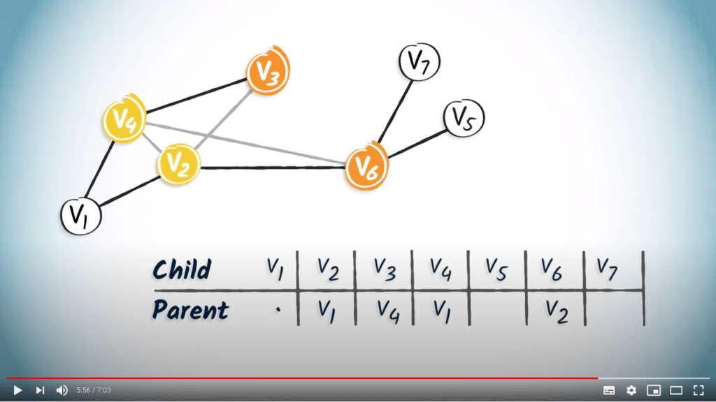
L’unique enfant de $v_4$ est $v_3$, et l’unique enfant de $v_2$ est $v_6$.
Ensuite, $v_6$ a deux enfants, $v_7$ et $v_5$. La table de routage est complète.
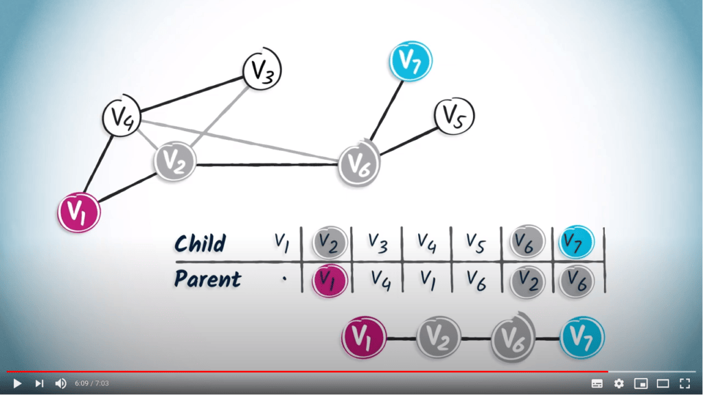
Si nous lisons le chemin de $v_1$ à $v_7$ dans la table, nous obtenons $(v_7, v_6, v_2, v_1)$.
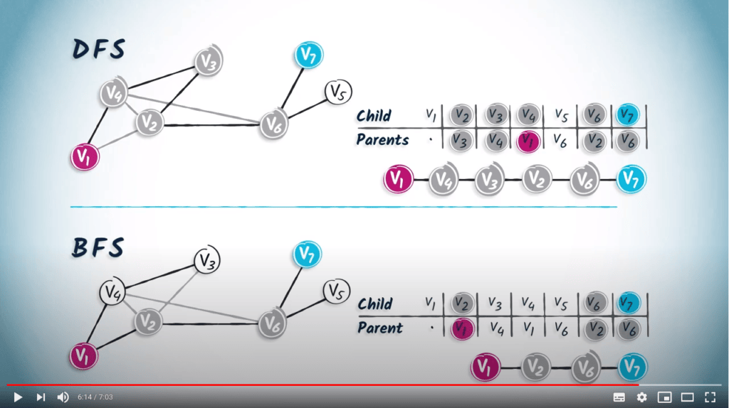
Nous pouvons voir que ce chemin est plus court que celui obtenu en utilisant un DFS, qui était $(v_7, v_6, v_2, v_3, v_4, v_1)$. C’est une différence importante entre DFS et BFS. BFS est une approche plus prudente que DFS, car BFS augmente progressivement la distance depuis la position de départ.
En utilisant BFS, nous pouvons être absolument certains de trouver le chemin le plus court entre deux sommets.
C’est tout pour aujourd’hui. Merci pour votre attention ! J’ai vraiment apprécié parler de routage avec vous.
Vous devez vous rappeler qu’il ne suffit pas de construire l’arbre couvrant pour naviguer entre les sommets du graphe, mais qu’il vous faut également un algorithme de routage.
À bientôt pour de nouvelles aventures algorithmiques !
2 — Implémentation des tables de routage
Pour implémenter des tables de routage dans un langage de programmation, vous avez besoin d’une structure de données qui peut vous aider à associer les sommets à leurs parents le long du parcours. Dans l’article sur comment représenter les graphes en mémoire, vous avez étudié quelques-unes de ces structures. Avec un peu d’imagination, toutes ces structures peuvent être utilisées pour implémenter des tables de routage. Voici quelques pistes :
-
Tableaux ou listes – Numérotez arbitrairement les sommets du graphe de 1 à $n$. Utilisez un tableau de taille $n$, ou une liste initialisée avec $n$ entrées égales à 0 (ou toute valeur en dehors de l’intervalle $[1, n]$). Ensuite, pour indiquer que le sommet à l’index $i$ est un prédécesseur du sommet à l’index $j$, il suffit de placer $i$ dans l’entrée $j$ de la structure. Plus tard, pour récupérer le chemin, il sera nécessaire de convertir les indices en sommets réels pour obtenir le chemin.
-
Dictionnaires – L’utilisation de dictionnaires est un peu plus directe, car ce sont des structures qui peuvent directement associer des variables à d’autres. Ainsi, il n’est pas nécessaire de numéroter les sommets. Par conséquent, pour indiquer que $v_1$ est un prédécesseur de $v_2$, il suffit d’associer la valeur $v_1$ à la clé $v_2$ dans la structure.
Pour aller plus loin
Il semble que cette section soit vide !
Y a-t-il quelque chose que vous auriez aimé voir ici ? Faites-le nous savoir sur le serveur Discord ! Peut-être pouvons-nous l’ajouter rapidement. Sinon, cela nous aidera à améliorer le cours pour l’année prochaine !
Pour aller encore plus loin
Il semble que cette section soit vide !
Y a-t-il quelque chose que vous auriez aimé voir ici ? Faites-le nous savoir sur le serveur Discord ! Peut-être pouvons-nous l’ajouter rapidement. Sinon, cela nous aidera à améliorer le cours pour l’année prochaine !