Algorithme de Dijkstra

Bonjour et bienvenue dans cette leçon sur l’algorithme de Dijkstra ! Cette semaine, nous allons parler des chemins les plus courts dans les graphes pondérés. Les algorithmes de parcours de graphe que nous avons déjà vus dans la leçon précédente ne peuvent pas être directement appliqués pour trouver les chemins les plus courts dans les graphes pondérés.

Pour illustrer pourquoi les algorithmes de parcours de graphe déjà présentés ne fonctionnent pas nécessairement pour les graphes pondérés, considérons le graphe jouet suivant.

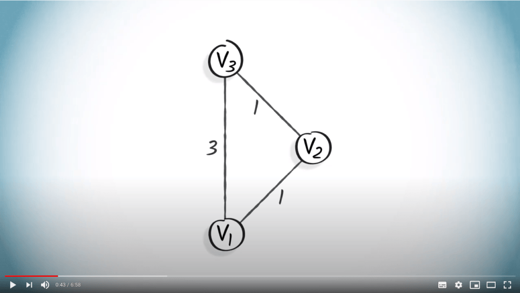
Ici, une recherche en largeur (BFS), en partant du sommet $v_1$, ne produira pas un arbre couvrant des chemins les plus courts. Par exemple, le chemin le plus court réel de $v_1$ à $v_3$ est $(\{v_1,v_2\}, \{v_2,v_3\})$, alors que le chemin trouvé en utilisant un BFS est $(\{v_1,v_3\})$.

Cela est dû au fait qu’un BFS favorise un plus petit nombre de sauts à partir du sommet initial, indépendamment des poids.

Pour résoudre ce problème, nous introduisons l’algorithme de Dijkstra. L’algorithme de Dijkstra est une modification du BFS qui nous permet de trouver les chemins les plus courts, même en présence de poids, si ceux-ci sont non négatifs.

Une petite note sur les poids. Jusqu’à présent dans ce MOOC, nous n’avons considéré que des poids non négatifs. Dans certains cas, il pourrait être pertinent d’ajouter des poids négatifs.

Par exemple, imaginez un chauffeur de taxi qui peut voyager entre des villes. Parfois, il gagne de l’argent parce qu’il a un client et parfois il en perd parce qu’il voyage seul. Nous pourrions donc considérer un graphe dont les sommets représentent des villes et les arêtes sont pondérées par le coût du voyage correspondant. Certains poids seraient alors positifs et d’autres négatifs.

Revenons aux graphes avec des poids non négatifs. La façon la plus simple de décrire l’algorithme de Dijkstra est d’imaginer le sommet de départ comme un robinet d’où l’eau s’écoule. L’eau progressera le long des sommets et traversera le graphe avec une vitesse inversement proportionnelle aux poids des arêtes, atteignant ainsi les sommets les plus proches en premier.

En d’autres termes, l’algorithme de Dijkstra est un algorithme de parcours dans lequel les sommets sont visités par distance croissante à partir du sommet initial.

À chaque étape, l’algorithme de Dijkstra stocke deux types d’informations :

1. quels sommets ont déjà été explorés ; et
2. une approximation des distances de $v_1$ à tous les autres sommets du graphe.

L’algorithme de Dijkstra répète deux étapes. À l’étape 1, il sélectionne un sommet non exploré $v$ qui est à une distance minimale de $v_1$. À l’étape 2, il met à jour les distances de $v_1$ vers les autres sommets du graphe, en utilisant les informations sur $v$ et ses voisins.

Notez que l’algorithme produit toujours un arbre couvrant des chemins minimaux dans le graphe, à condition que les poids soient non négatifs. Nous n’allons pas prouver ce résultat ici, mais ce serait un excellent exercice si vous souhaitez approfondir les concepts décrits dans cette leçon.

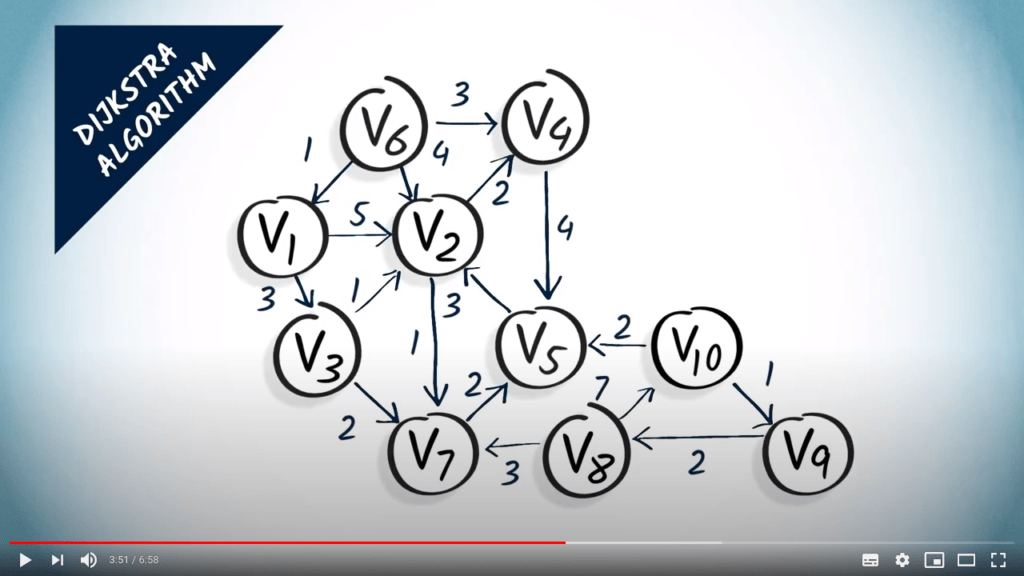
Décrivons plus précisément comment fonctionne l’algorithme de Dijkstra à l’aide de l’exemple suivant. Nous allons construire un arbre couvrant minimal en partant du sommet $v_1$ dans ce graphe.

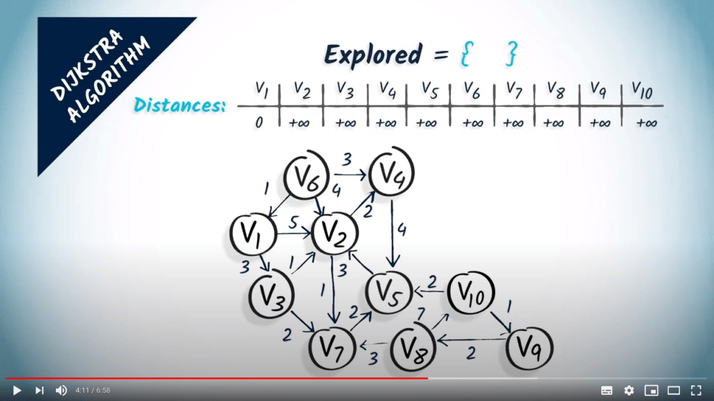
Nous initialisons deux structures de données : Premièrement, l’ensemble des sommets explorés, qui est initialement vide. Deuxièmement, le tableau des distances de $v_1$ vers les autres sommets du graphe, initialisé à $+\infty$ partout sauf pour $v_1$, où nous insérons un 0.

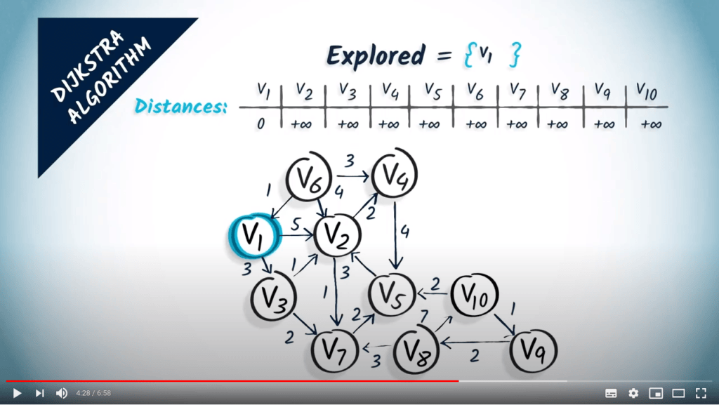
La première étape consiste à sélectionner un sommet non exploré qui est à une distance minimale du sommet de départ. Ici, nous sélectionnons $v_1$ comme sommet de départ et l’ajoutons à l’ensemble des sommets explorés.

La deuxième étape consiste à mettre à jour les distances en tenant compte du sommet sélectionné $v_1$ et de ses voisins. Ici, $v_1$ a deux voisins : $v_2$ et $v_3$. Les atteindre en un saut depuis $v_1$ coûte respectivement 5 et 3. Nous mettons donc à jour nos distances depuis $v_1$ en disant que $v_2$ est à une distance de 5 et $v_3$ à une distance de 3. Notez que la longueur d’un chemin le plus court de $v_1$ à $v_2$ est en réalité 4, mais nous ne pouvons pas encore le déterminer uniquement à partir des résultats de l’algorithme.

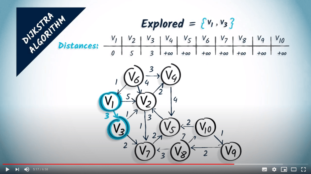
Commençons maintenant une nouvelle itération de l’algorithme. À la première étape, nous sélectionnons un sommet non exploré à une distance minimale de $v_1$. Ici, nous choisissons $v_3$, qui est à une distance de 3. Nous l’ajoutons à l’ensemble des sommets explorés.

À la deuxième étape, nous examinons les voisins de $v_3$, qui sont $v_2$ et $v_7$, avec des poids correspondants de 1 et 2. Ainsi, si nous voulons atteindre $v_2$ en passant par $v_3$ un saut avant, nous avons un coût total de 3, qui est le coût pour aller à $v_3$, plus 1, qui est le coût d’un saut de $v_3$ à $v_2$. Cela est meilleur que la distance précédente estimée pour $v_2$, donc nous modifions les distances en conséquence. En ce qui concerne $v_7$, nous avons maintenant une distance estimée de 3, le coût pour aller à $v_3$ plus 2, qui est le coût d’un saut de $v_3$ à $v_7$.

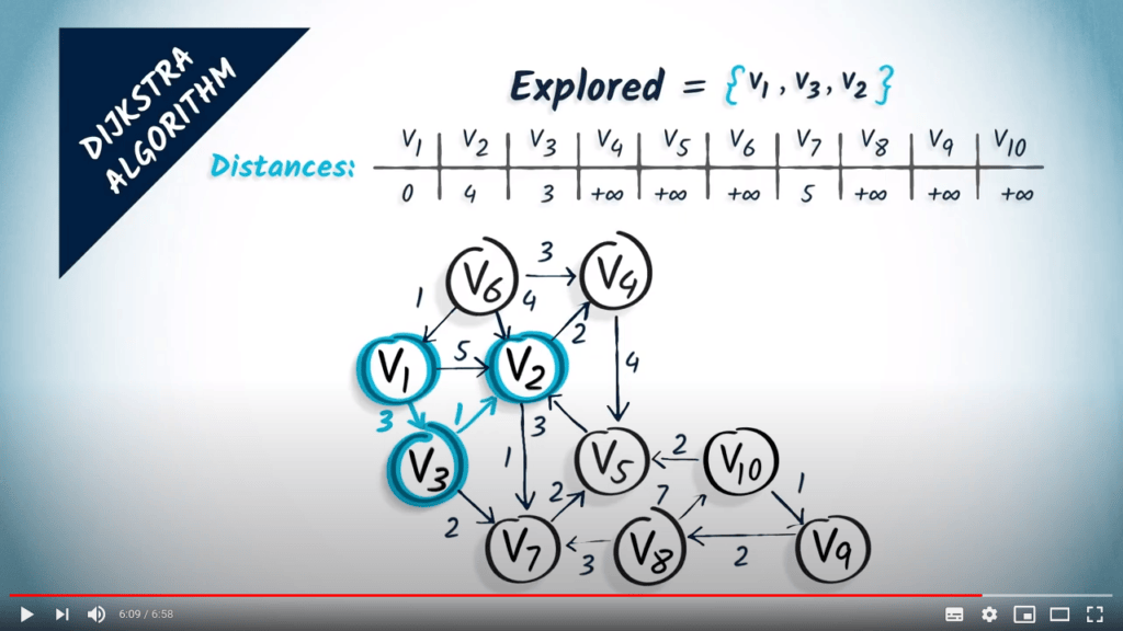
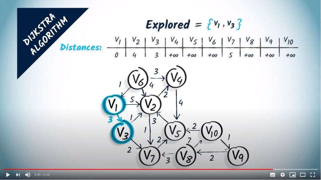
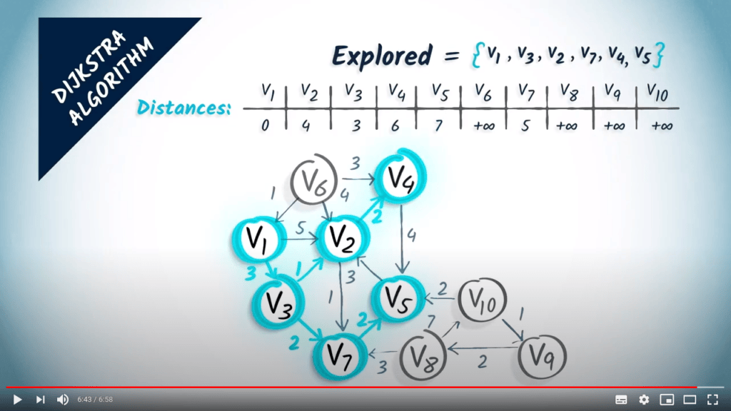
Une nouvelle itération commence. Maintenant, nous sélectionnons le prochain sommet non exploré avec la plus petite distance, qui est $v_2$. Nous l’ajoutons à l’ensemble des sommets explorés.

Le sommet $v_2$ a deux voisins, $v_4$ et $v_7$. Le sommet $v_4$ est estimé à une distance de $4 + 2 = 6$, et $v_7$ à une distance de $4 + 1 = 5$. Nous mettons donc à jour la distance vers $v_4$. En ce qui concerne $v_7$, la nouvelle distance trouvée n’est pas meilleure que l’ancienne, donc elle n’a aucun effet.

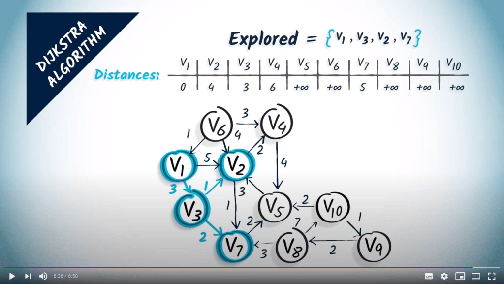
Une nouvelle itération commence. Nous sélectionnons $v_7$ à une distance de 5 et l’ajoutons à la liste des sommets explorés. Et ainsi de suite…

Finalement, nous obtenons l’arbre couvrant suivant.

C’est tout pour cette leçon ! Ensuite, nous verrons comment implémenter l’algorithme de Dijkstra en utilisant des tas minimaux.