Complexité des problèmes & NP-complétude
Temps de lecture10 minEn bref
Résumé de l’article
Jusqu’à présent, nous avons étudié la complexité des algorithmes, comme moyen d’estimer le temps nécessaire à leur exécution en fonction de leurs entrées. Plus généralement, les problèmes ont une notion de complexité. Cela signifie que pour un problème donné, il n’existe pas d’algorithme avec une meilleure complexité pour le résoudre.
À retenir
-
Il existe des classes de complexité pour les problèmes.
-
La complexité d’un problème décrit la complexité minimale d’un algorithme qui le résout.
-
Il existe des intersections, des relations d’inclusion ou des équivalences entre certaines classes de complexité.
-
La complexité peut également décrire la mémoire nécessaire pour résoudre un problème.
Contenu de l’article
1 — Vidéo
Veuillez consulter la vidéo ci-dessous (en anglais, affichez les sous-titres si besoin). Nous fournissons également une traduction du contenu de la vidéo juste après, si vous préférez.
Information
Cliquez ici pour afficher la traduction de la vidéo.

Bonjour ! Vous êtes de retour ? Super ! Cela signifie que vous n’avez pas encore eu assez de complexité !
Aujourd’hui, explorons ce que sont les problèmes P et NP, et comment cela impacte la résolution des problèmes.
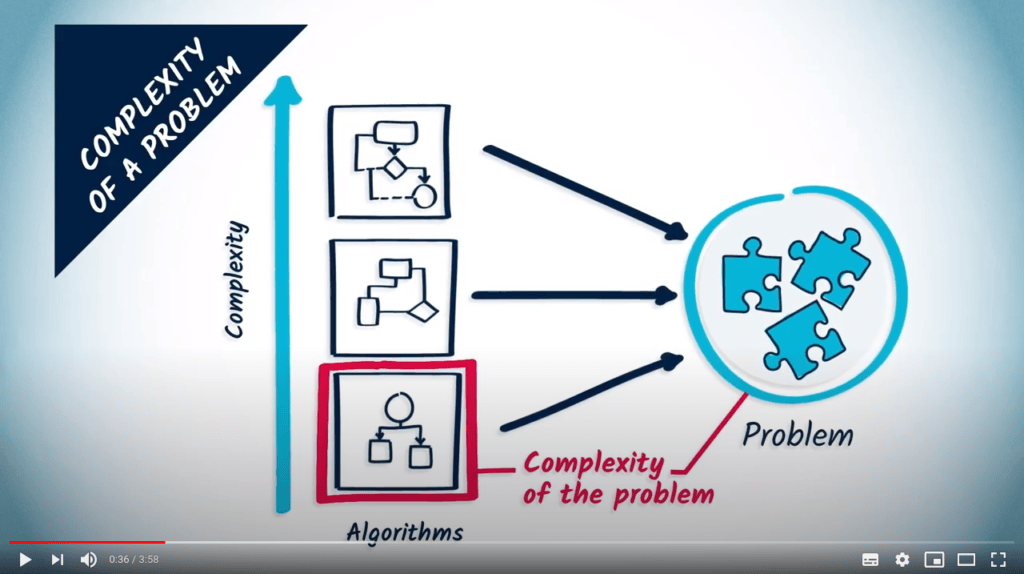
La complexité d’un problème est liée à la complexité des algorithmes. La complexité d’un problème est définie comme la complexité minimale des algorithmes qui le résolvent.

Comme nous l’avons vu la semaine dernière, la complexité d’un algorithme inclut une connotation de “pire cas”, car elle mesure le “maximum” d’opérations élémentaires nécessaires à son exécution.
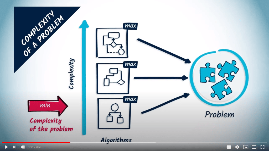
Par conséquent, la complexité d’un problème, qui est intuitivement la complexité du “meilleur” algorithme possible pour le résoudre, peut être vue comme un “minimum d’un maximum”.
Certains problèmes sont plus difficiles à résoudre que d’autres, dans le sens où ils nécessitent des algorithmes plus complexes pour être résolus.
Comme je vais vous le montrer aujourd’hui, différentes classes de complexité ont été définies pour décrire la difficulté de résolution d’un problème.
Dans cette optique, un problème est dit “polynomial” s’il peut être résolu par un algorithme dont la complexité est asymptotiquement dominée par un polynôme.
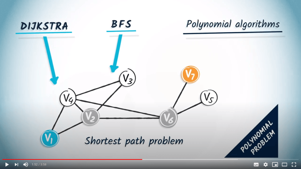
Nous avons déjà rencontré de nombreux algorithmes polynomiaux dans ce cours, tels que Dijkstra ou le BFS. Ainsi, si nous considérons, par exemple, les problèmes de plus court chemin que ces algorithmes résolvent, ils peuvent être facilement identifiés comme des problèmes polynomiaux, car un algorithme polynomial les résout.
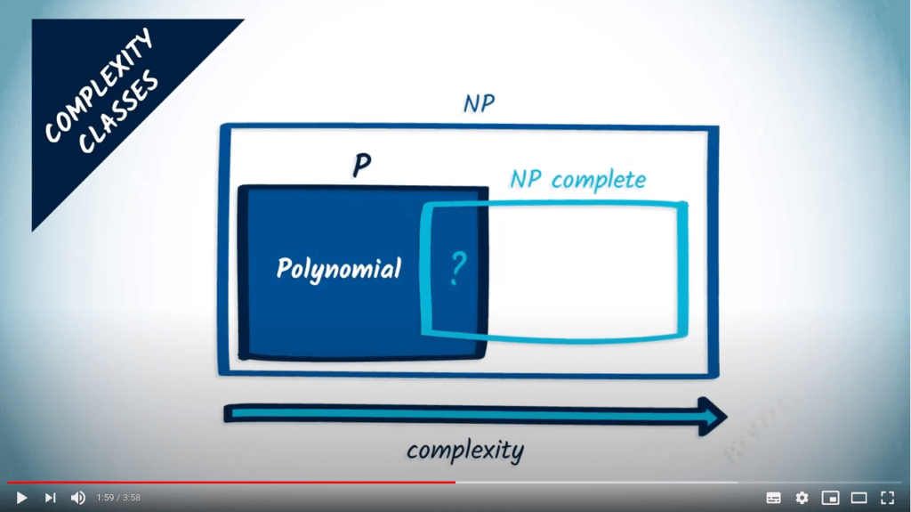
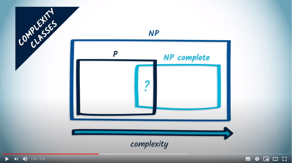
En conséquence, tous ces problèmes appartiennent à la classe de complexité appelée P, qui signifie Polynomial.
Pour d’autres problèmes, il est plus difficile de déterminer leur classe de complexité. C’est le cas du TSP, par exemple. Personne n’a réussi à trouver un algorithme polynomial pour le résoudre, et il y a de fortes suspicions que cela soit tout simplement impossible.
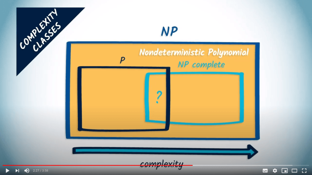
Le TSP appartient donc à une classe de problèmes plus difficiles, appelés problèmes NP pour “Nondeterministic Polynomial”. En gros, un problème de décision est un problème NP si nous pouvons vérifier “rapidement”, avec une complexité polynomiale, si une solution candidate est effectivement une solution.
Sans entrer dans trop de détails, nous devons souvent utiliser des algorithmes avec une complexité exponentielle pour résoudre les problèmes NP.
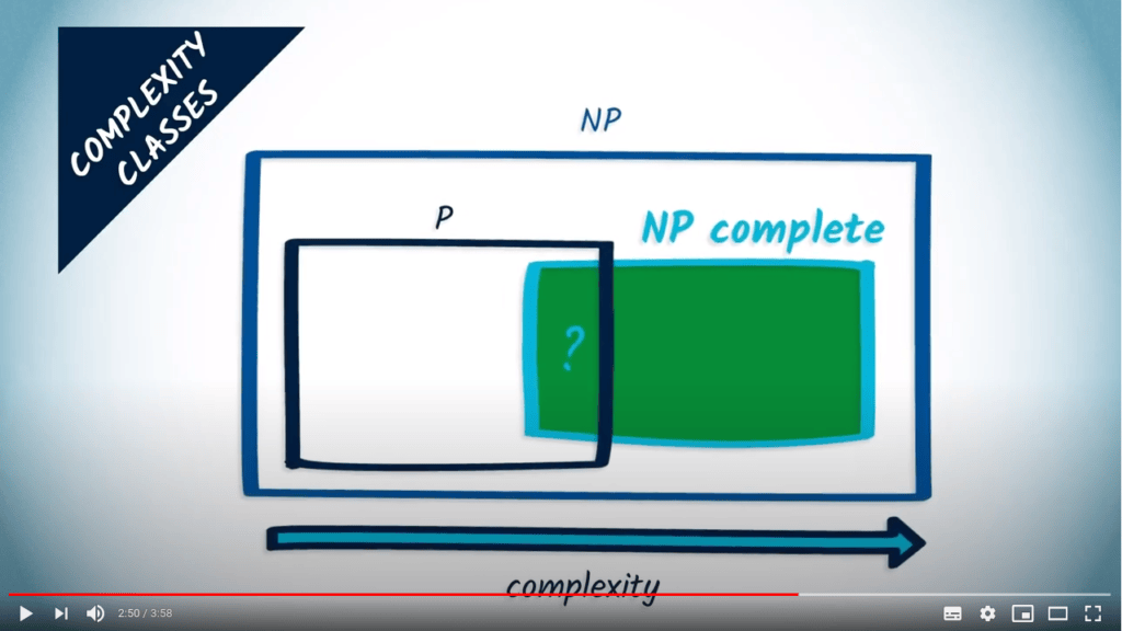
Une autre classe célèbre de problèmes est celle des problèmes NP-Complets. Les problèmes NP-Complets sont au moins aussi difficiles à résoudre que tous les autres problèmes NP. En d’autres termes, un algorithme capable de résoudre un problème NP-Complet peut résoudre n’importe quel autre problème NP.
Il suffirait de réécrire les entrées et de réinterpréter les sorties pour les adapter au nouveau problème. Ces réécritures peuvent être effectuées à l’aide d’algorithmes polynomiaux.
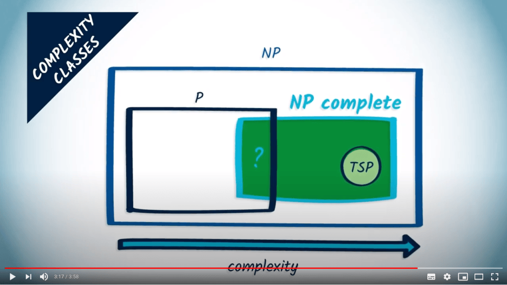
Comme vous l’avez peut-être deviné, il a été prouvé que le TSP est un problème NP-Complet.
Ainsi, aujourd’hui, je vous ai montré que si vous êtes capable de résoudre le TSP, vous êtes également capable de résoudre n’importe quel autre problème NP. D’un point de vue théorique, cela semble intéressant, mais d’un point de vue opérationnel, résoudre le TSP nécessite encore un algorithme exponentiel, ce qui, pour notre jeu de labyrinthe, n’est probablement pas idéal. Ne vous laissez pas décourager, car la semaine prochaine, nous vous montrerons comment résoudre le problème plus rapidement, à condition d’accepter que la solution ne soit pas nécessairement optimale, mais suffisamment bonne.
Pour aller plus loin
2 — Complexité en espace
Les classes de complexité ci-dessus décrivent les besoins en temps pour résoudre les problèmes. Afin de mesurer d’autres besoins, tels que la consommation de mémoire, il existe d’autres classes de complexité.
Similaire à la complexité en temps, la complexité en espace mesure la plus petite quantité de mémoire qu’un programme aurait besoin pour résoudre le problème en question, pour le pire cas d’entrée. Encore une fois, cela peut être vu comme un “minimum de maximum”.
Nous utilisons également les notations grand-O pour décrire l’utilisation de la mémoire, en fonction de la taille de l’entrée. Par exemple, $O(n)$ désigne une utilisation linéaire de la mémoire, et $O(n!)$ indique que résoudre le problème nécessite au moins une quantité de mémoire qui croît de manière factorielle avec la dimension de l’entrée.
Comme pour les classes de complexité en temps, il existe une énorme taxonomie des classes de complexité en espace.
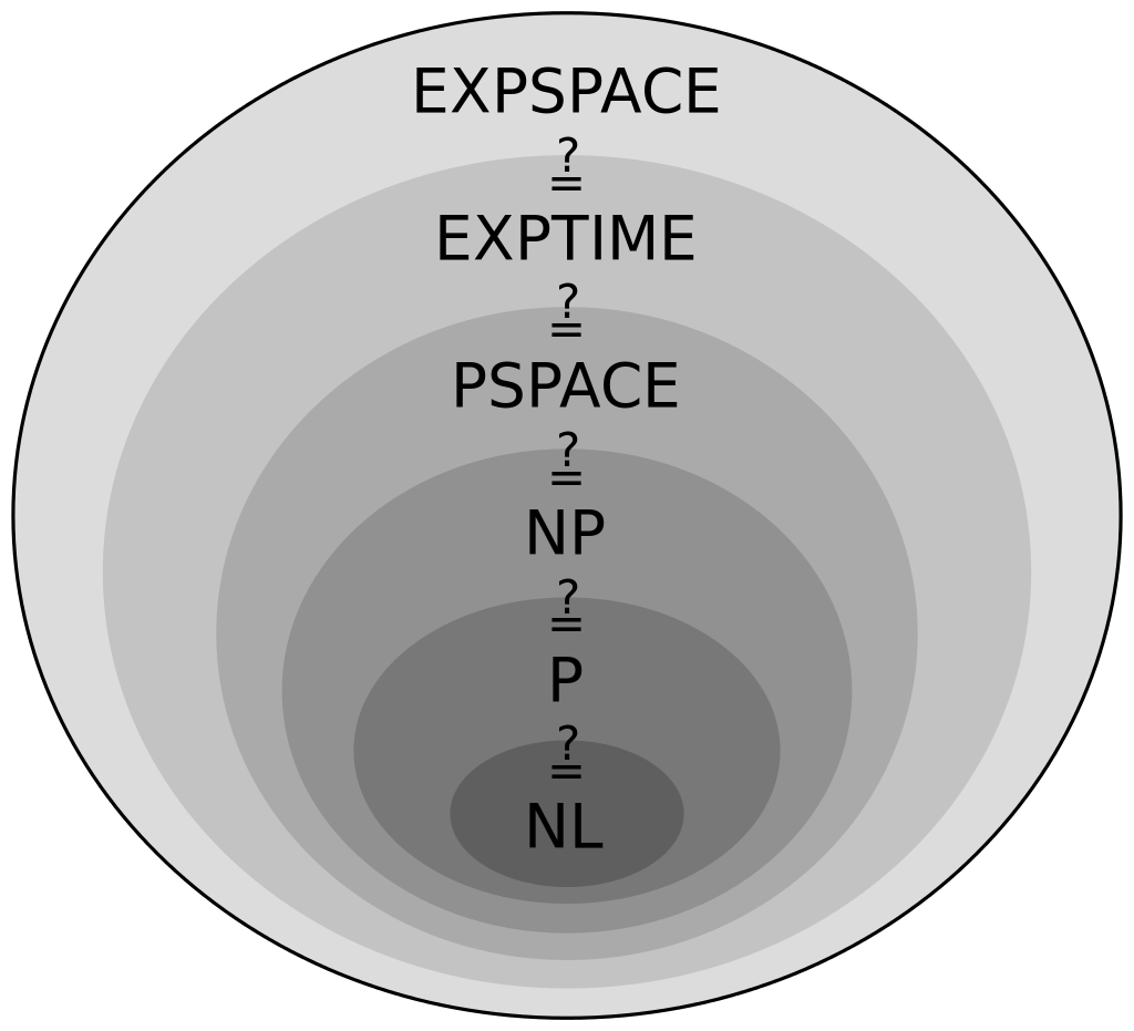
Parmi les classes classiques, PSPACE indique qu’un problème ne peut pas être résolu avec moins qu’une quantité polynomiale de mémoire.
Les complexités en espace et en temps ne sont pas indépendantes. Par exemple, il est montré que NP $\subseteq$ PSPACE. Cependant, il existe de nombreuses égalités entre classes qui sont inconnues, dont beaucoup sont des problèmes ouverts en recherche depuis des décennies.
Pour aller encore plus loin
-
A taxonomy of complexity classes of functions.
Plein d’informations sur les différentes classes de complexité.
-
Le problème de déterminer si P et NP sont identiques est un problème majeur en informatique.