Solutions approchées
Temps de lecture25 minEn bref
Résumé de l’article
Comme mentionné dans les autres articles, les heuristiques fournissent des solutions approchées. Ici, nous donnons plus de détails sur la façon de caractériser la qualité d’une telle solution. En particulier, nous nous concentrerons sur la correction et le gain temporel.
À retenir
-
Une solution approchée est un compromis entre qualité de la solution et temps requis pour l’obtenir.
-
Les solutions qui sont des compromis optimaux de plusieurs critères sont appelées Pareto-optimales.
Contenu de l’article
1 — Vidéo
Veuillez consulter la vidéo ci-dessous (en anglais, affichez les sous-titres si besoin). Nous fournissons également une traduction du contenu de la vidéo juste après, si vous préférez.
Information
Cliquez ici pour afficher la traduction de la vidéo.

Nous revoici. Ravi de voir que vous êtes arrivé(e)s à la semaine 5 ! Aujourd’hui, nous parlerons de la comparaison des implémentations. Face à des problèmes pratiques comme le problème du voyageur de commerce, le TSP, nous préférerions évidemment une solution qui est à la fois rapidement obtenue, et correcte.

Dans le cas des problèmes NP-Complets, ce qui est le cas pour le TSP, nous savons que ce n’est tout simplement pas possible. Nous devons sacrifier la rapidité, la correction, ou un peu des deux.
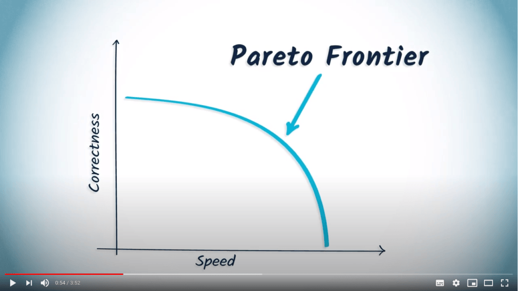
Ce type de compromis est souvent appelé “frontière de Pareto”, que nous pouvons définir de la manière suivante : “quel est l’algorithme le plus rapide que nous pouvons trouver pour résoudre un problème avec un niveau de correction donné ?”.
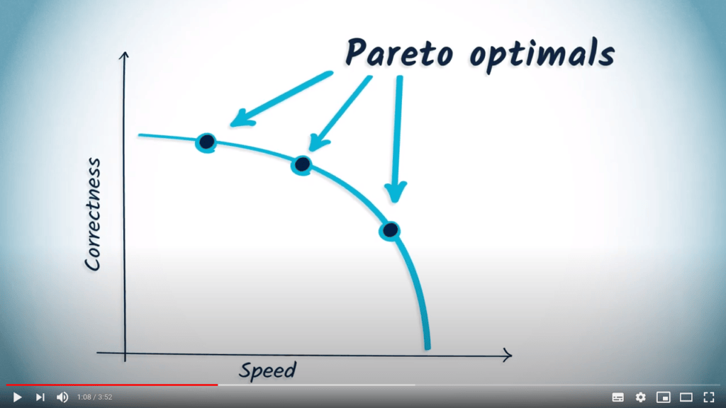
Nous appelons “optimum de Pareto” un point qui se trouve sur une frontière de Pareto, ce qui signifie qu’il correspond à un compromis optimal entre rapidité et correction.
Un optimum de Pareto est typiquement un optimum qui dépend de l’importance relative de deux paramètres ou plus, comme la taille du problème que nous traitons.
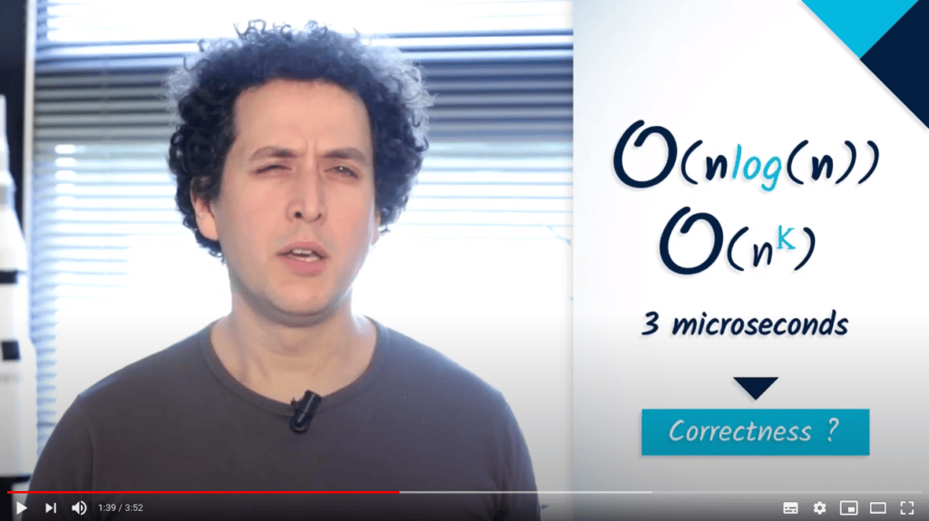
Définissons quelques notions liées à la mesure de la rapidité et de la correction. Nous pouvons mesurer la rapidité d’un algorithme en utilisant la complexité ou des mesures de temps d’exécution. Mais la correction d’un algorithme est difficile à définir, ce qui rend sa mesure difficile.
Pour le TSP, nous savons que nous voulons trouver un chemin le plus court, et donc la correction pourrait simplement être mesurée comme un écart par rapport à la longueur du chemin le plus court.
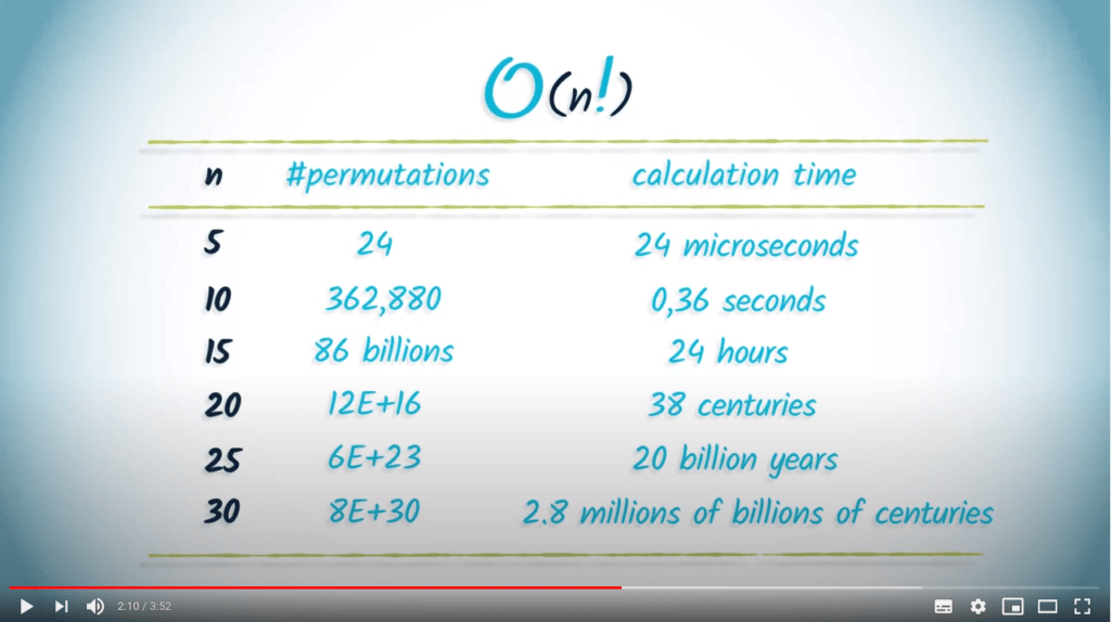
Mais en pratique, ce n’est pas toujours aussi simple. Trouver le chemin le plus court peut être impossible s’il y a plus que quelques dizaines de sommets, car nous avons vu que la complexité d’une recherche exhaustive croît exponentiellement. Cela signifie que la correction d’un algorithme approchant une solution pour le TSP est très difficile à estimer.
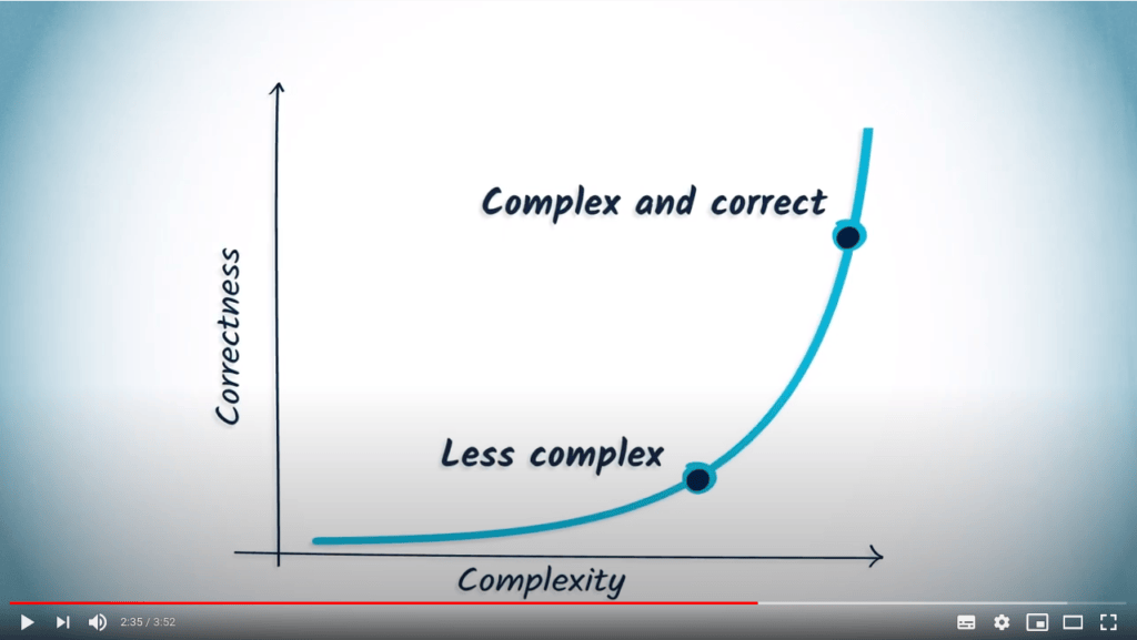
Ce que nous savons, c’est que plus nous avons de complexité à gérer, meilleure devrait être la solution en termes de correction. Dans le pire des cas, nous pouvons toujours nous rabattre sur une solution moins complexe qui a déjà été proposée.
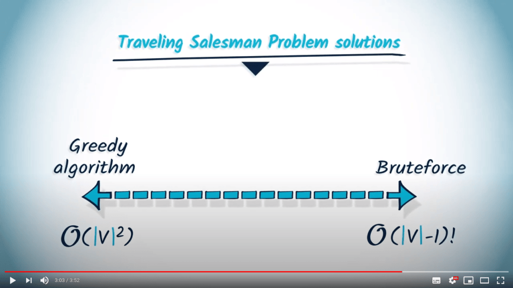
Reprenons le TSP comme exemple. Il existe de nombreuses étapes intermédiaires entre l’algorithme glouton, qui consiste à toujours cibler la ville la plus proche suivante, et celui de bruteforce, qui examine exhaustivement tous les chemins possibles pour visiter chaque ville. Trouver un intermédiaire entre ces deux extrêmes ne devrait être envisagé que s’ils apportent réellement des améliorations en termes de complexité.
Pour déterminer si une solution proposée est efficace, vous devez toujours la comparer avec une approche simple, tant en termes de correction que de complexité. Si votre solution doit être 10 fois plus complexe pour apporter une amélioration de 1% en termes de correction, peut-être que cela ne vaut pas l’effort, sauf si cette amélioration de 1% fait une différence significative par rapport aux autres solutions.
Eh bien, c’est tout pour aujourd’hui, merci pour votre attention ! C’est ma dernière vidéo. J’ai vraiment aimé enseigner pour vous ! Je vous laisse en de bonnes mains pour la semaine 6, durant laquelle Patrick et Vincent vous parleront de la théorie des jeux combinatoires. Au revoir !
Pour aller plus loin
2 — Exemple de la coloration de graphes
2.1 — L’algorithme exact
Prenons l’exemple suivant : nous appelons “coloration d’un graphe” un vecteur d’entiers, chacun associé à l’un de ses sommets. Ces entiers sont appelés couleurs de sommet, et peuvent être identiques.
Une coloration est dite “propre” si tous les sommets reliés par une arête sont de couleurs différentes. Le “nombre chromatique d’un graphe” est le nombre minimum de couleurs qui apparaissent dans une coloration spécifique.
Ce problème est un exemple connu de problème NP-Complet. Une façon de le résoudre avec précision est de lister toutes les colorations possibles à 1 couleur, puis à 2 couleurs, etc. jusqu’à trouver une coloration propre.
Le code Python suivant résout le problème comme décrit ci-dessus :
Dans cet exemple, un graphe est implémenté sous la forme d’une liste de listes. Il contient 6 sommets (nommés $v_1$ à $v_6$), et 8 arêtes (symétriques). La solution retournée par l’algorithme est :
Cela indique que trois couleurs suffisent pour avoir une coloration propre du graphe, avec :
- $v_1$ et $v_4$ partageant la couleur 0.
- $v_2$ et $v_5$ partageant la couleur 1.
- $v_3$ et $v_6$ partageant la couleur 2.
2.2 — L’approche gloutonne
Cet algorithme est très complexe et une solution approchées bien connue consiste à trier les sommets par nombre décroissant de voisins, en les coloriant dans cet ordre en choisissant la plus petite couleur positive qui laisse la coloration propre. Cet algorithme approché est décrit ci-dessous :
Cet algorithme est beaucoup moins complexe que le précédent, et permet donc de considérer des graphes avec beaucoup plus de sommets. Ici, nous obtenons le résultat suivant :
Notez qu’ici, nous trouvons le même résultat que l’algorithme exhaustif. Cependant, ce n’est pas toujours le cas.
2.3 — Simulations
Afin d’évaluer la qualité de notre algorithme approché, nous nous concentrerons sur deux choses : le temps de calcul et la précision. Pour tester ces deux quantités, nous allons faire la moyenne des résultats sur un grand nombre de graphes aléatoires.
Afin d’automatiser un peu les choses, nous allons adapter nos codes pour prendre des arguments en ligne de commande et produire un fichier exploitable. Créons deux fichiers Python.
Le programme suivant, measure_greedy.py, retourne le temps d’exécution moyen de l’approche gloutonne pour résoudre le problème considéré, ainsi que le nombre moyen de couleurs nécessaires pour un graphe de taille fixe :
De même, le programme suivant measure_exhaustive.py évalue la solution exhaustive :
Nous pouvons maintenant exécuter les commandes suivantes pour lancer les deux algorithmes sur des graphes aléatoires (100 graphes par ordre de graphe). La recherche exhaustive ne sera évaluée que sur un sous-ensemble des ordres de graphe en raison de considérations de temps :
Comparons les temps d’exécution en utilisant Libreoffice :
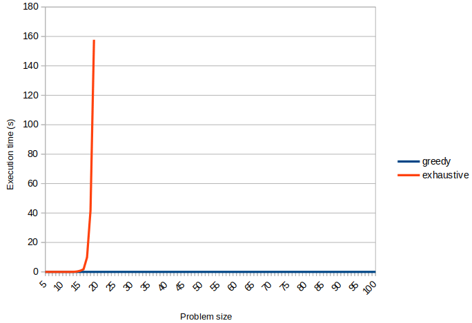
Clairement, le gain en temps d’exécution est significatif. De même, comparons les nombres chromatiques moyens trouvés pour les deux algorithmes :
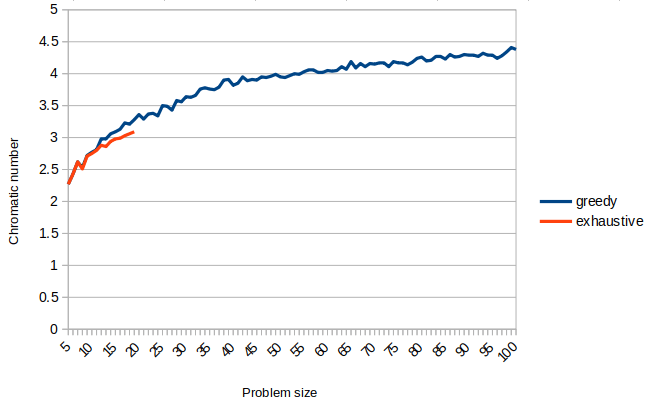
En regardant la courbe de précision, il semble que la perte de précision n’est pas très élevée, du moins pour les tailles de problème qui ont pu être calculées en utilisant l’approche exhaustive. Pour des graphes plus grands, nous ne pouvons pas calculer la solution exacte en raison de la complexité pour la trouver.
Afin d’évaluer un peu plus cet aspect, nous allons évaluer les solutions trouvées en utilisant l’approche gloutonne sur des graphes bipartis, pour lesquels nous savons que le nombre chromatique est toujours 2 :
Nous obtenons les résultats suivants :
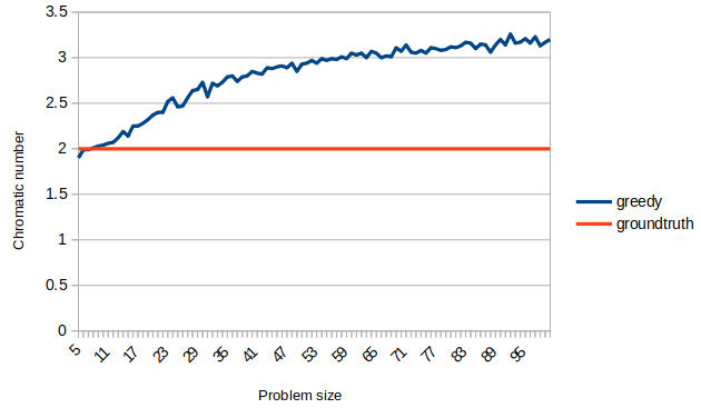
Ici encore, le résultat semble raisonnable, ce qui nous amène à penser que cette heuristique est bien adaptée au problème.
Vous devriez tout de même noter que pour de petites tailles de problème, le nombre chromatique trouvé est parfois inférieur à 2, ce qui semble erroné. Cependant, notez que le générateur de graphes aléatoires ne vérifie pas la connexité du graphe, ce qui peut conduire à des graphes à plusieurs composantes connexes.
Pour aller encore plus loin
-
Ici, nous avons étudié les compromis temps/précision, mais c’est un concept plus général.
-
Si vous voulez en savoir plus sur ces graphes particuliers.