Activité pratique
Durée2h30Consignes globales
Dans cette activité, vous allez développer un algorithme heuristique pour approximer une solution au TSP. Ici, nous nous concentrons sur un algorithme glouton.
Dans les parties optionnelles, nous suggérons quelques heuristiques alternatives et améliorations. La partie sur 2-OPT n’est pas très difficile, et intéressante à tester. N’hésitez pas à y jeter un œil !
Contenu de l’activité
1 — L’algorithme glouton
1.1 — Préparation
À faire
Avant de commencer, créez les fichiers nécessaires dans votre workspace PyRat en suivant les instructions ci-dessous.
-
players/Greedy.py– Initialisez un nouveau joueur via une classeGreedyqui hérite de la classePlayer. -
games/visualize_Greedy.py– Créez un fichier qui démarrera une partie avec un joueurGreedy, dans un labyrinthe avec de la boue (mud_percentage), et 20 morceaux de fromage (nb_cheese). -
tests/test_Greedy.py– Créez un fichier de tests unitaires pour votre joueurGreedy.
Important
Comme pour la séance précédente, ce n’est pas grave si vous travaillez avec un labyrinthe qui ne contient pas de boue si vous êtes en retard sur l’algorithme de Dijkstra. Néanmoins, notez que pour le dernier livrable, cela ne sera plus accepté.
1.2 — Programmer l’algorithme glouton
Nous voulons utiliser l’heuristique suivante : le chemin le plus court qui passe par tous les morceaux de fromage peut être approximé en allant successivement vers le morceau de fromage le plus proche.
Afin d’écrire un algorithme glouton avec cette heuristique, suivez les étapes ci-dessous, comme pour la séance précédente.
À faire
Identifiez les méthodes nécessaires pour le joueur.
Vous devriez d’abord identifier les méthodes dont vous aurez besoin.
N’hésitez pas à revenir aux articles que vous deviez étudier pour aujourd’hui.
Une fois identifiées, écrivez leurs prototypes dans votre fichier joueur Greedy.py.
À faire
Identifiez les tests pour valider ces méthodes.
Déterminez quels tests vous devriez effectuer pour garantir que les méthodes du joueur fonctionnent comme prévu.
Écrivez les prototypes des méthodes réalisant ces tests dans votre fichier de tests unitaires test_Greedy.py.
À faire
Programmez les méthodes du joueur et les tests.
Plus tard dans cette activité pratique, nous demandons que vous changiez l’heuristique utilisée par votre algorithme glouton. Donc, assurez-vous de réfléchir attentivement aux fonctions que vous identifiez, i.e., n’écrivez pas tout dans une seule méthode !
La vidéo suivante vous montre un exemple de ce que vous devriez observer :
1.3 — Comparer avec l’algorithme exhaustif
Comme vous l’avez vu dans les articles à étudier, un algorithme approché est un compromis entre précision, complexité, et parfois d’autres propriétés (mémoire requise, besoin de matériel spécifique…).
Comparons le temps nécessaire pour récupérer tous les morceaux de fromage, pour le joueur Greedy que vous venez de créer, comparé aux joueurs Exhaustive de la dernière séance.
À faire
Créez un script dans le sous-répertoire games, qui créera (pour chacun de ces joueurs) une courbe du nombre de tours nécessaires pour attraper tous les fromages, en fonction de leur nombre dans le labyrinthe.
Évidemment, vous ne devriez pas aller très haut en termes de nombre de morceaux de fromage pour le joueur Exhaustive.
De plus, il serait intéressant de tracer des résultats moyennés sur plusieurs parties, car il peut y avoir de la variabilité entre les parties.
1.4 — Un glouton réactif
Jusqu’à présent, vous avez probablement suivi le même raisonnement que dans les séances précédentes.
En d’autres termes, la façon la plus directe de programmer l’algorithme glouton est de calculer le chemin dans preprocessing, et de le dérouler à chaque appel de turn.
Maintenant, imaginons que vous ayez un adversaire dans le jeu. Si vous suivez un tel chemin prédéterminé sans considérer que votre adversaire peut manger certains morceaux de fromage entre-temps, vous allez sûrement perdre. En effet, vous allez essayer d’aller chercher des morceaux de fromage qui ont disparu, tandis que l’adversaire se concentrera sur ceux qui restent.
1.4.1 — Une première amélioration
Repensons comment fonctionne l’algorithme glouton :
- Considérez que vous êtes sur une case particulière du labyrinthe, et vous exécutez votre algorithme glouton.
- La sortie devrait être une liste de morceaux de fromage à manger, triée dans l’ordre dans lequel les obtenir.
- Vous vous dirigez donc vers le premier morceau de fromage de cette liste.
Toutefois, au lieu de calculer cette liste une seule fois au début du jeu, vous pouvez la recalculer chaque fois que vous atteignez un morceau de fromage. Cela permet de s’adapter aux changements dans le labyrinthe, tels que les morceaux de fromage qui ont été mangés par l’adversaire.
À faire
Créez un nouveau joueur player/GreedyEachCheese.py, qui réalise cette amélioration.
Créez également un script games/visualize_GreedyEachCheese.py pour lancer une partie avec celui-ci.
N’oubliez pas d’ajouter des tests unitaires supplémentaires dans un fichier dédié si nécessaire.
1.4.2 — Encore mieux
Le joueur GreedyEachCheese a encore un inconvénient.
En effet, si l’adversaire récupère le morceau de fromage vers lequel nous nous dirigeons, nous terminerons quand même notre trajectoire.
Afin de le rendre encore plus réactif, repensons notre GreedyEachCheese :
- Considérez que vous êtes sur une case particulière du labyrinthe, et vous exécutez votre algorithme glouton.
- La sortie devrait être le prochain morceau de fromage à récupérer (appelons-le
c). - Une fois que vous avez déterminé
c, vous effectuez une action dans sa direction.
Eh bien, si nous faisons un pas dans la direction de c, nous pouvons distinguer les deux scénarios suivants :
cest toujours là – Alors,cest toujours le morceau de fromage le plus proche, car nous avons réduit le nombre de tours nécessaires pour y aller de 1 (ou plus s’il y avait de la boue). Nous devrions continuer dans sa direction.ca été attrapé par un adversaire – Alors, nous devrions nous concentrer sur un autre morceau de fromage.
Notez que nous pouvons satisfaire les deux scénarios en exécutant notre algorithme glouton à chaque tour pour déterminer la prochaine action (et non le prochain morceau de fromage comme GreedyEachCheese).
En faisant cela, nous trouverions le même chemin à suivre si le fromage est toujours là, et nous déplacerions ailleurs si nécessaire.
À faire
Créer un nouveau joueur players/GreedyEachTurn.py, qui réalise cette amélioration.
Créez également un script games/GreedyEachTurn.py pour lancer une partie avec celui-ci.
N’oubliez pas d’ajouter des tests unitaires supplémentaires dans un fichier dédié si nécessaire.
1.4.3 — Comparer les programmes
Vous avez maintenant trois algorithmes gloutons. Essayons de les comparer pour voir si les améliorations apportées ont un impact sur les résultats.
À faire
Créez un script de jeu à deux équipes games/match_Greedy_GreedyEachTurn.py pour faire s’affronter Greedy contre GreedyEachTurn.
Pour ce faire, inspirez-vous du script games/sample_game.py.
Vous devriez faire démarrer les joueurs à des emplacements aléatoires en utilisant un code similaire à celui-ci :
Sinon, les deux joueurs commenceront au milieu du labyrinthe, et suivront les mêmes trajectoires.
À faire
En moyenne sur 100 parties, quel joueur gagne ? De combien de parties ? Est-ce significatif ?
Pour ce faire, vous pouvez utiliser un T-test pour un échantillon pour vérifier si la liste des différences de scores a (ou non) une moyenne de 0.
À faire
Créez également un autre script de jeu games/match_GreedyEachCheese_GreedyEachTurn.py pour faire s’affronter GreedyEachCheese contre GreedyEachTurn.
À faire
Est-il intéressant d’exécuter l’algorithme glouton à chaque tour comparé à chaque morceau de fromage (du point de vue des résultats) ? S’il y a une amélioration, est-elle significative ?
Pour aller plus loin
2 — 2-opt
Il existe de nombreux autres algorithmes approchés que vous pouvez utiliser pour approximer la solution au TSP. Nous pouvons distinguer deux catégories :
- Solution unique – Une seule solution au problème TSP est trouvée, puis éventuellement améliorée pour obtenir une meilleure solution. L’algorithme glouton entre dans cette catégorie.
- Solutions multiples – De nombreuses solutions sont trouvées et mélangées pour produire de meilleures solutions. Les algorithmes génétiques entrent dans cette catégorie.
L’algorithme glouton construit une solution unique et l’utilise ensuite. Il n’effectue aucune amélioration de cette solution, bien que certaines faciles pourraient être faites.
Une heuristique simple pour s’appuyer sur le résultat glouton est 2-opt. L’algorithme partira d’une solution particulière au TSP (soit aléatoire soit construite avec un algorithme glouton), et l’améliorera progressivement en supprimant les routes qui se croisent.
À faire
Essayez de coder cette heuristique en suivant les indications sur la page Wikipedia sur 2-opt, ou d’autres ressources.
3 — Factoriser les codes
Si vous avez développé d’autres heuristiques, vous pouvez maintenant essayer de factoriser votre code.
À faire
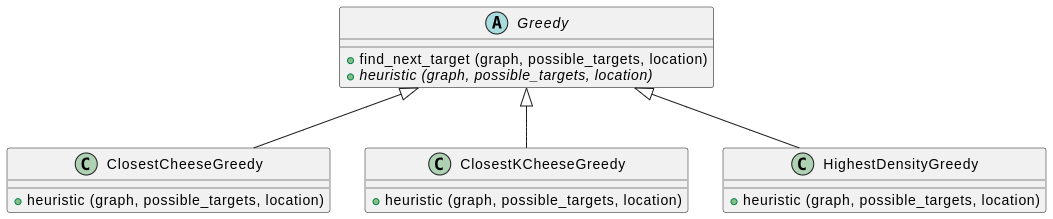
Une solution est d’avoir une classe abstraite utils/GreedyHeuristic (dans un sous-répertoire utils), et des classes enfants qui encodent les heuristiques.
Enfin, créez un joueur players/GreedyPlayer.py qui exploite l’heuristique gloutonne que vous souhaitez.
Voici un petit diagramme UML qui représente une factorisation possible. Consultez la séance 2 pour un guide sur comment le lire.
4 — Une autre heuristique
Jusqu’à présent, votre heuristique était de favoriser le morceau de fromage le plus proche. Voici deux heuristiques possibles que vous pouvez implémenter :
À faire
Meilleurs $k$ morceaux de fromage – Favoriser le morceau de fromage c de sorte que la série de $k$ morceaux de fromage commençant par c soit la plus courte.
Pour ce faire, vous pouvez résoudre un TSP jusqu’à la profondeur $k$.
À faire
Zones de haute densité – Favoriser les morceaux de fromage qui sont situés dans des zones où il y a beaucoup de fromage.
Pour ce faire, vous devez calculer une mesure de densité pour chaque fromage.
5 — Réutiliser les parcours
Vous avez peut-être déjà remarqué que vous exécutez plusieurs fois l’algorithme de Dijkstra au cours du jeu. Parfois, vous utilisez même l’algorithme plusieurs fois à partir du même endroit. Cela peut arriver par exemple lorsque vous exécutez l’algorithme à partir d’une position que vous avez déjà visitée plus tôt dans le jeu, ou lors du calcul d’une heuristique à partir d’un morceau de fromage.
Puisque c’est une opération coûteuse, il peut être judicieux de stocker les résultats dans un attribut pour éviter de recalculer les tables de routage si vous l’avez déjà fait. C’est une approche que vous avez vue en cours, appelée mémoïsation
Une solution rapide est de créer un attribut et de vérifier d’abord son contenu avant d’exécuter le code coûteux.
À faire
Essayez de l’implémenter dans votre joueur glouton en utilisant le code ci-dessous comme guide.
Pour aller encore plus loin
6 — Recherche locale
La recherche locale est une méta-heuristique qui explore l’espace des solutions comme un parcours dans un graphe. L’idée est que nous allons créer un graphe de solutions dynamiquement, et l’explorer jusqu’à ce que nous soyons bloqués dans un optimum local. Plus en détail, ce que vous pouvez faire pour implémenter une recherche locale est :
-
Partir d’une solution donnée $s$.
-
Identifier toutes les solutions voisines de $s$. Pour ce faire, vous devez définir une opération qui, lorsqu’elle est appliquée à $s$, générera de nouvelles solutions. Par exemple, vous pourriez permuter deux sommets dans la solution. Cela générera une solution voisine pour chaque paire de sommets.
-
Évaluer les voisins, et votre nouveau $s$ devient la meilleure solution parmi les voisins.
-
Boucler jusqu’à ce qu’aucun voisin ne soit meilleur que $s$.
À faire
Essayez différentes stratégies pour générer des voisins. Vous pouvez également essayer différentes stratégies d’exploration des voisins, inspirées par des algorithmes tels que BFS ou DFS.
7 — Recuit simulé
Le recuit simulé est une méthode efficace pour approximer le TSP. Comme pour la recherche locale, vous avez besoin d’une méthode pour générer des voisins. Vous pouvez ensuite appliquer le recuit simulé comme suit :
-
Partir d’une solution initiale $s$.
-
Initialiser le recuit simulé :
- Définir la température initiale $T$.
- Choisir une stratégie de décroissance de température, par exemple, décroissance exponentielle $T = T * \alpha$ où $\alpha$ est légèrement inférieur à 1 (par exemple, 0.99).
- Définir un critère d’arrêt, tel qu’un nombre maximum d’itérations ou une température minimale.
-
Pour chaque itération :
- Générer une nouvelle solution $s’$ en modifiant légèrement $s$.
- Calculer la différence de qualité $\delta$ entre $s$ et $s’$.
- Si $s’$ est meilleure, l’accepter.
- Si $s’$ est moins bonne, l’accepter avec une probabilité dépendant de la température actuelle et de la différence de coût. Cette probabilité est calculée comme $P = exp\left(-\frac{\delta}{T}\right)$.
- Réduire la température selon la stratégie de décroissance.
-
Arrêter lorsque la température est suffisamment basse ou après un nombre prédéfini d’itérations.
À faire
Essayez d’implémenter le recuit simulé pour le TSP en utilisant les étapes ci-dessus comme guide.