Activité pratique
Durée2h30Consignes globales
Dans cette activité, vous devrez développer une solution pour récupérer plusieurs morceaux de fromage en un minimum d’actions. Pour cela, nous allons programmer une recherche exhaustive, puis la compléter avec une stratégie de backtracking.
Si vous souhaitez aller plus loin, nous vous conseillons de jeter un œil à la partie sur les solveurs. Vous y découvrirez des concepts supplémentaires intéressants.
Contenu de l’activité
1 — L’algorithme exhaustif
1.1 — Préparation
À faire
Avant de commencer, créez les fichiers nécessaires dans votre workspace PyRat en suivant les instructions ci-dessous.
-
players/Exhaustive.py– Dupliquez le fichierTemplatePlayer.pyet renommez-le enExhaustive.py. Ensuite, renommez la classe enExhaustive. -
games/visualize_Exhaustive.py– Créez un fichier qui lancera une partie avec un joueurExhaustive, dans un labyrinthe avec de la boue (argumentmud_percentage) et 5 morceaux de fromage (argumentnb_cheese). Vous pouvez éventuellement définir unrandom_seedet unetrace_length. -
tests/test_Exhaustive.py– En vous inspirant des fichierstest_DFS.py,test_BFS.pyettest_Dijkstra.pyvus lors des sessions précédentes, créez un fichiertest_Exhaustive.py. Ce fichier contiendra les tests unitaires que vous développerez pour tester les méthodes de votre joueurExhaustive.
Information
Dans cette activité pratique, vous devrez utiliser un algorithme de parcours à un moment donné. Si vous n’avez pas réussi à faire fonctionner un algorithme de Dijkstra, vous pouvez retirer la boue du labyrinthe et utiliser un parcours en largeur (BFS) à la place. Cela vous permettra de travailler sur l’activité pratique. Plus tard, vous pourrez essayer de remplacer votre BFS par l’algorithme de Dijkstra pour étendre vos résultats aux graphes pondérés.
1.2 — Programmer l’algorithme exhaustif
Pour écrire un algorithme exhaustif, suivez les mêmes étapes que la dernière fois. Commençons par les méthodes pour découper notre problème en sous-problèmes plus petits.
À faire
Identifiez d’abord les méthodes nécessaires.
N’hésitez pas à revenir aux articles que vous deviez étudier pour aujourd’hui.
Une fois identifiées, écrivez leurs prototypes (i.e., la ligne def xxx (...): et un contenu égal à pass) dans votre fichier joueur Exhaustive.py.
Maintenant que nous avons découpé le problème, réfléchissons aux tests unitaires nécessaires pour valider chaque méthode.
À faire
Identifiez les tests unitaires nécessaires pour chaque méthode.
N’hésitez pas à revenir aux fichiers de tests des sessions précédentes pour vous inspirer.
Une fois identifiés, écrivez leurs prototypes dans votre fichier de tests test_Exhaustive.py.
Maintenant que nous avons les prototypes des méthodes et des tests, nous pouvons implémenter tout ça.
À faire
Programmez les méthodes dans Exhaustive.py et les tests dans test_Exhaustive.py.
N’oubliez pas d’exécuter vos tests régulièrement pour vous assurer que tout fonctionne correctement.
Information
Identifier tous les chemins possibles dans un graphe complet peut se faire de plusieurs manières :
-
Parcours – Dans les articles, nous vous proposons une approche basée sur un parcours en profondeur (DFS). Cela est encore plus simple avec une implémentation récursive d’un DFS, comparée à celle réalisée lors de la séance 2. Cette approche a l’avantage de permettre d’intégrer des optimisations à différentes étapes de la recherche.
-
Permutations – Chaque chemin dans le graphe complet correspond à une permutation de sommets (et vice versa). Vous pouvez donc facilement itérer sur toutes les permutations possibles, en utilisant par exemple la bibliothèque Python
itertools. Cette solution est plus simple à programmer, mais ne vous permettra pas d’ajouter un backtracking dans votre recherche (voir plus bas). Nous vous suggérons donc d’utiliser cette approche uniquement si vous rencontrez trop de difficultés avec l’autre.
La vidéo suivante montre un exemple de ce que vous devriez observer :
Une fois votre programme fonctionnel, essayez d’augmenter le nombre de morceaux de fromage.
À faire
Quel est le nombre maximum de morceaux de fromage que vous pouvez atteindre en un temps raisonnable ?
1.3 — Ajouter du backtracking
1.3.1 — Améliorations de la recherche exhaustive
Nous allons maintenant ajouter une stratégie de backtracking à notre recherche exhaustive. L’idée est de couper certaines branches de l’arbre d’exploration lorsque nous savons qu’elles ne mèneront pas à une meilleure solution que celle déjà trouvée.
On va donc essayer deux améliorations successives de notre algorithme exhaustif.
À faire
Créez un nouveau joueur players/Backtracking.py (copiez Exhaustive.py comme base), et une partie l’utilisant.
Ensuite, améliorez votre algorithme exhaustif en y intégrant une stratégie de backtracking.
La qualité de cette stratégie dépendra de la manière dont vous décidez de couper les branches. En effet, plus on trouve tôt une bonne solution, plus on peut couper de branches.
À faire
Créez un nouveau joueur players/SortedNeighbors.py (copiez Backtracking.py comme base), et une partie l’utilisant.
Réfléchissez à un ordre dans lequel il serait intéressant d’explorer les sommets, et mettez à jour vos codes pour que votre recherche en tienne compte.
Encore une fois, n’oubliez pas les tests !
1.3.2 — Évaluer vos améliorations
Vous avez maintenant trois programmes basés sur une recherche exhaustive. Il serait intéressant d’évaluer si vos améliorations accélèrent effectivement la résolution du TSP, ou si vos calculs supplémentaires nuisent aux performances.
À faire
Comparez le temps nécessaire aux différents programmes pour résoudre le TSP. Les indications ci-dessous vous donnent des idées sur la manière de procéder.
Pour mesurer le temps nécessaire pour résoudre le TSP, vous pouvez :
-
Tracer le temps moyen (sur 100 parties par exemple) requis pour terminer une partie, en fonction du nombre de morceaux de fromage dans le labyrinthe.
-
Pour un nombre fixe de morceaux de fromage, calculer les distributions des temps nécessaires pour chaque programme. Ensuite, utilisez des tests statistiques adaptés pour évaluer si les distributions sont significativement différentes.
Information
Assurez-vous d’exécuter vos expériences avec un Python qui désactive les assertions, car celles-ci seraient comptées dans le temps d’exécution.
Pour cela, exécutez le fichier Python avec python3 -O games/votre_script.py.
À faire
Comparez le nombre de branches coupées et restantes dans votre exploration. Voici quelques idées pour y parvenir.
Pour comparer les branches, vous pouvez :
-
Adapter votre code pour compter combien de branches ont été coupées lors de l’exploration. Un graphique intéressant que vous pourriez produire est le nombre de branches coupées, en fonction de leur profondeur dans l’arbre (c’est-à-dire, le nombre de sommets dans le chemin avant la coupure). En effet, plus tôt vous coupez une branche, moins vous avez de branches complètes à explorer, et donc plus l’algorithme sera rapide.
-
Adapter votre code pour compter combien de branches complètes ont été explorées. Un graphique intéressant que vous pourriez produire est le nombre de branches complètes explorées de longueur au plus $l$, en fonction de la longueur $l$.
À faire
À l’aide de ces indicateurs, quelle est la qualité de votre stratégie de tri dans SortedNeighbors.py ?
Pour aller plus loin
2 — Factoriser les codes
Dans les parties précédentes, nous vous avons demandé plusieurs fois de copier le fichier précédent comme base. Il en résulte probablement que vous avez plusieurs fois la même fonction dans ces fichiers, ce qui est problématique. En effet, si vous trouvez une erreur dans une telle fonction maintenant, vous devrez mettre à jour plusieurs endroits dans vos codes. C’est une surcharge de travail inutile, et vous pourriez ajouter de nouvelles erreurs en le faisant mal.
À faire
En vous inspirant des séances précédentes, essayez de factoriser vos différentes recherches exhaustives.
Voici deux choses possibles que vous pouvez faire (choisissez votre préférée) :
-
Bibliothèque – Vous pouvez créer un fichier Python externe (par exemple appelé
tsp_utils.py) et y écrire vos fonctions dupliquées. Ensuite, mettez à jour vos joueurs pour importer les fonctions nécessaires depuis ce fichier. -
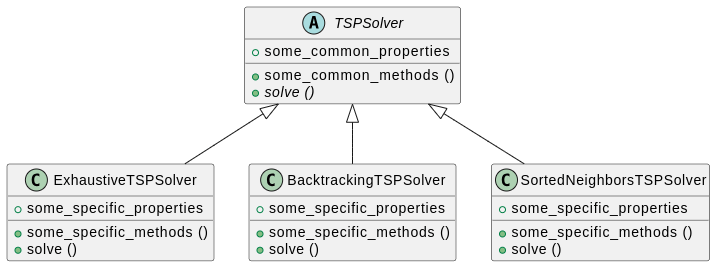
Classe – Vous pouvez créer une classe abstraite
TSPSolver(dans un répertoireutils), qui regroupe les méthodes communes à tous les solveurs exhaustifs. Ensuite, écrivez les classesExhaustiveTSPSolver,BacktrackingTSPSolveretSortedNeighborsTSPSolverqui héritent deTSPSolver. Enfin, créez un joueurTSPPlayer.pyqui utilise le solveur souhaité.Voici un petit diagramme UML représentant une factorisation possible. Consultez la séance 2 pour un guide sur la lecture de celui-ci.
3 — L’algorithme de branch-and-bound
Alors que le backtracking est une optimisation basée sur un algorithme DFS, l’algorithme de branch-and-bound repose sur une approche de type BFS. Cet algorithme vous a été présenté dans la section optionnelle d’un article que vous deviez étudier pour aujourd’hui.
À faire
Essayez de l’implémenter dans un nouveau joueur appelé BranchAndBoundTSPSolver.
Comment se compare-t-il à vos autres joueurs ?
Pour aller encore plus loin
4 — Solveurs
4.1 — Intuition des améliorations possibles
Il peut sembler étrange que nous ayons du mal à trouver la solution du TSP dans un graphe avec aussi peu de sommets que 10-15, alors que des outils comme les GPS, les planificateurs de trajets, etc., existent. En pratique, la plupart de ces outils reposent sur ce que nous appelons des “heuristiques”, qui trouvent des solutions approximatives (et non exactes). Vous étudierez de telles approches lors de la prochaine session.
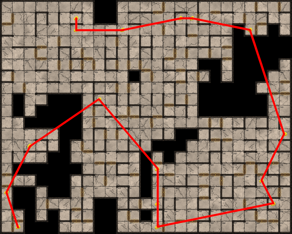
Cependant, il reste encore des possibilités d’amélioration avec des algorithmes exacts. En effet, nous pouvons facilement penser à des améliorations simples. Par exemple, c’est probablement une mauvaise décision de faire des allers-retours dans le labyrinthe comme suit :

Attraper des morceaux de fromage proches est évidemment mieux que cette approche. Par exemple, cette permutation est nettement plus courte (bien qu’elle ne soit pas nécessairement la meilleure) :
Vous pouvez voir cette optimisation comme une sorte d’inégalité triangulaire. En effet, le méta-graphe qui représente la répartition des morceaux de fromage dans le labyrinthe est une matrice de distances avec des propriétés particulières. Cette propriété (et de nombreuses autres) sont exploitées par des outils avancés appelés “solveurs”.
4.2 — Qu’est-ce qu’un solveur ?
Un solveur est un outil générique qui, pour un problème donné, explore l’espace des solutions de manière intelligente. En effet, les solutions peuvent être organisées dans un espace abstrait, et leur proximité dans cet espace indique une similarité entre les solutions. Vous pouvez voir cela comme un graphe de solutions, et les solveurs exploreront ce graphe intelligemment pour trouver la solution optimale.
Nous n’entrerons pas dans les détails sur le fonctionnement des solveurs, mais voici un lien sur comment le formaliser mathématiquement si vous êtes intéressé(e).
4.3 — Utilisons un solveur
À faire
Essayez d’utiliser un solveur pour résoudre le TSP sur un labyrinthe PyRat.
En Python, vous pouvez par exemple utiliser la bibliothèque ORTools.
Pour l’utiliser, vous devez définir une matrice de distances qui modélise votre problème. Ensuite, adaptez l’exemple fourni par ORTools pour résoudre le TSP sur un labyrinthe PyRat.
Avec cette solution, vous devriez être capable de calculer la solution du TSP pour un grand nombre de morceaux de fromage dans le temps alloué à la fonction preprocessing(...).