Tas min
Temps de lecture15 minEn bref
Résumé de l’article
Dans cet article, vous apprendrez ce qu’est un tas min (min-heap), une structure de données avec des propriétés particulières. Elle sera très utile pour implémenter l’algorithme de Dijkstra.
À retenir
-
Les tas min sont des structures de données où les données sont extraites en fonction d’une valeur de référence.
-
Ils peuvent être utilisés pour implémenter facilement l’algorithme de Dijkstra.
-
Il existe plusieurs façons de programmer un tas min, certaines étant plus efficaces que d’autres.
-
En Python, la bibliothèque
heapqfournit une bonne implémentation des tas min.
Contenu de l’article
1 — Vidéo
Veuillez consulter la vidéo ci-dessous (en anglais, affichez les sous-titres si besoin). Nous fournissons également une traduction du contenu de la vidéo juste après, si vous préférez.
Important
Certaines “codes” apparaissent dans cette vidéo. Veuillez garder à l’esprit que ce sont des pseudo-codes, c’est-à-dire qu’ils ne sont pas écrits dans un langage de programmation réel. Ça ressemble à du Python, mais ça n’est pas du Python !
Leur but est simplement de décrire les algorithmes sans se soucier des détails de la syntaxe d’un langage de programmation particulier. Vous devrez donc effectuer un peu de travail pour les rendre pleinement fonctionnels en Python si vous souhaitez les utiliser dans vos programmes.
Information
Cliquez ici pour afficher la traduction de la vidéo.

Bienvenue à nouveau ! Ravi de vous revoir !
La semaine dernière, nous avons vu comment implémenter les algorithmes DFS et BFS en utilisant des structures de file. Cette semaine, pour implémenter l’algorithme de Dijkstra, nous allons avoir besoin d’une structure de file un peu plus élaborée : une structure qui prendra en compte les poids dans le graphe.

Jetons un coup d’œil à une autre structure de file pour implémenter l’algorithme de Dijkstra. Voici le tas min.
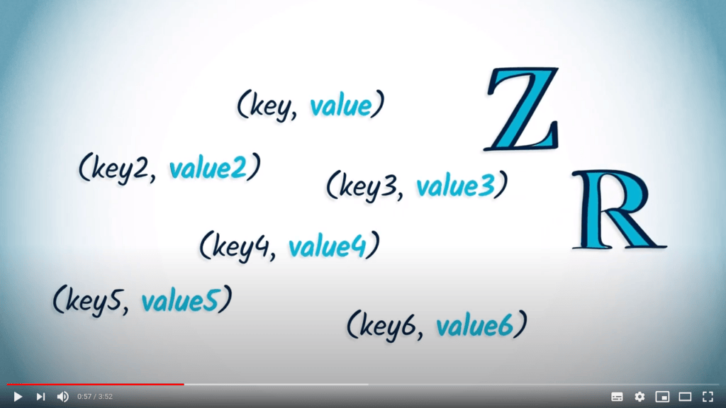
Un tas min est une structure de données dans laquelle les éléments sont stockés sous forme de couples (clé, valeur).
La valeur est une quantité qui doit appartenir à un ensemble totalement ordonné, par exemple, l’ensemble des entiers ou des nombres réels.
Avec un tas min, deux opérations élémentaires peuvent être effectuées.
La première est add_or_replace(...).
L’opération add_or_replace(...) est utilisée pour ajouter un couple (clé, valeur) au tas min.
Si la clé existe déjà, et que sa valeur associée est plus grande que celle que nous voulons ajouter, alors la valeur est mise à jour avec la nouvelle valeur.
Si la valeur est plus petite, alors l’opération est ignorée.
La deuxième opération élémentaire du tas min est remove(...), qui renverra le couple (clé, valeur) correspondant à la valeur minimale dans le tas min.
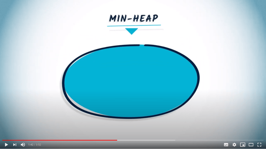
Illustrons l’utilisation d’un tas min avec un exemple. Nous initialisons un tas min vide.
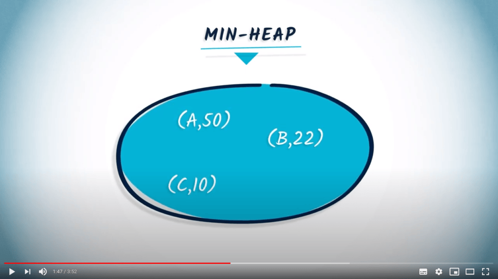
Ajoutons trois couples (clé, valeur) : $(A, 50)$, $(B, 22)$ et $(C, 10)$.
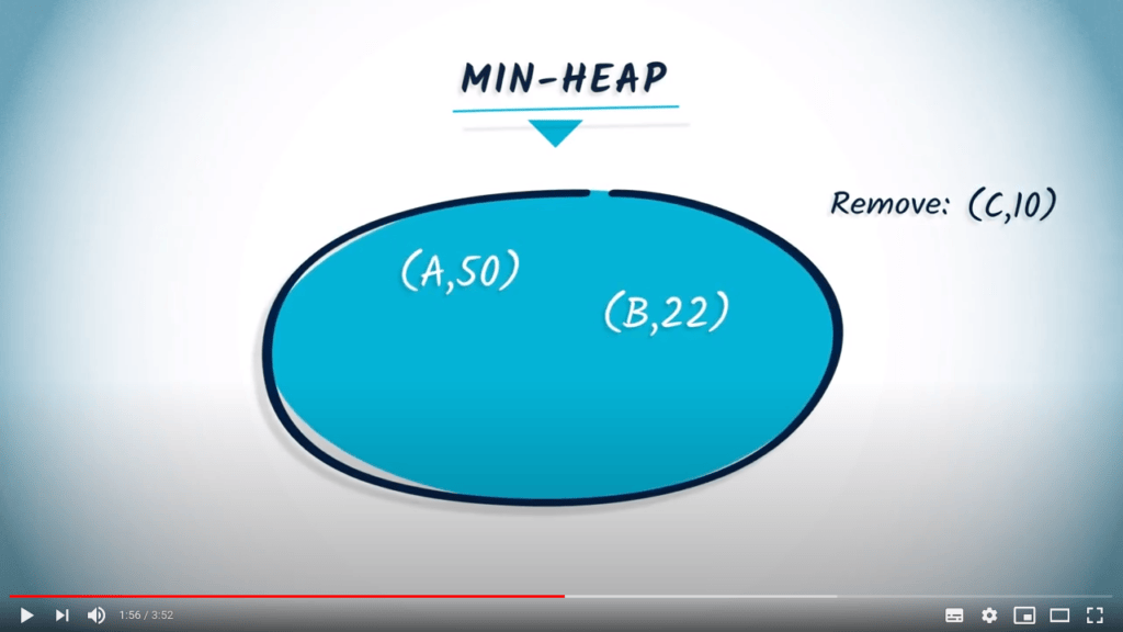
Retirons maintenant un élément de ce tas min avec remove(...).
Cette opération renverra $(C, 10)$, et l’état du tas min sera ${ (A, 50), (B, 22) }$.
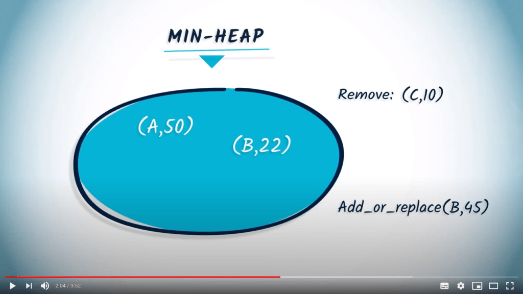
Maintenant, utilisons add_or_replace(...) avec le couple $(B, 45)$.
Comme 45 est plus grand que 22, rien ne se passe.
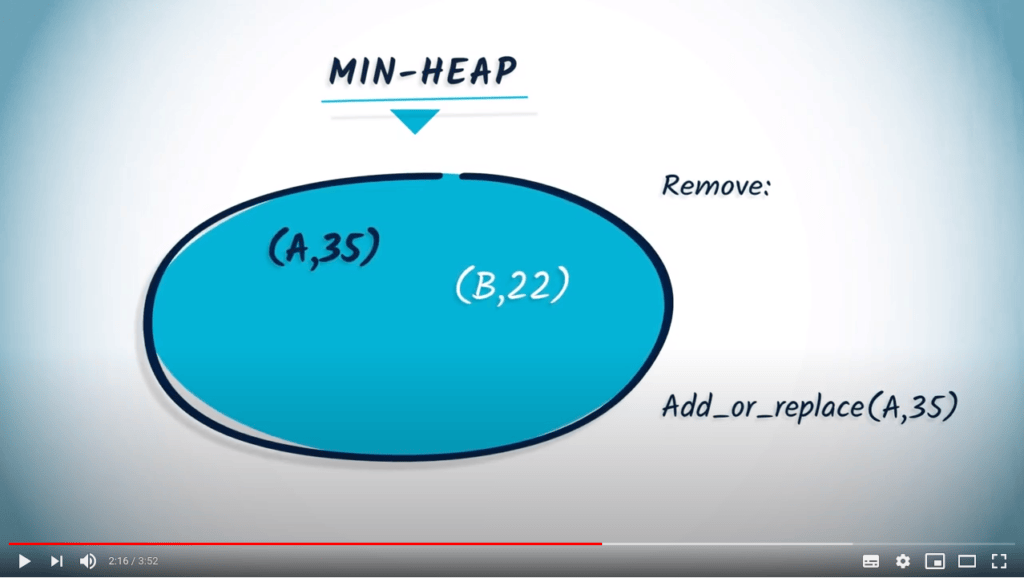
Maintenant, utilisons add_or_replace(...) avec le couple $(A, 35)$.
35 est plus petit que 50, et donc l’entrée correspondant à $A$ sera mise à jour, ce qui donne le tas min suivant.
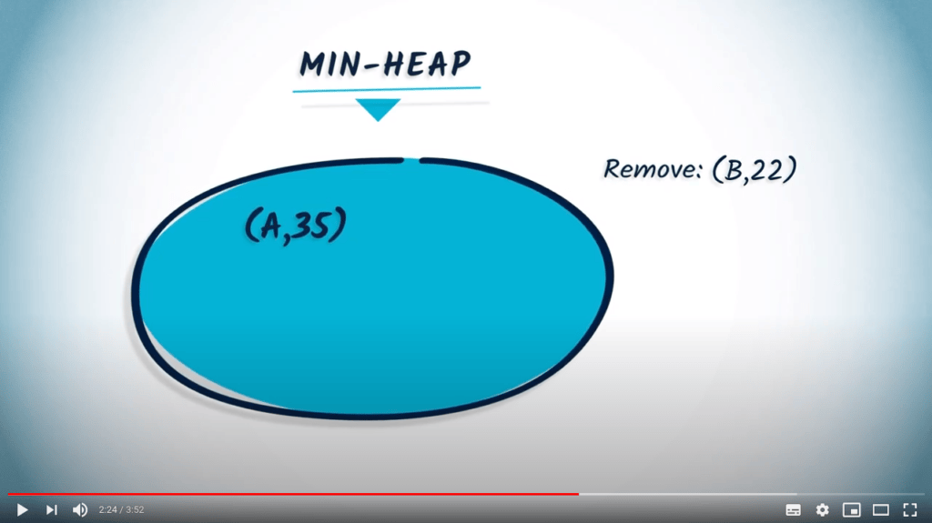
Enfin, retirons un élément du tas min avec remove(...).
Cela renverra $(B, 22)$, et mettra à jour le tas min comme suit.
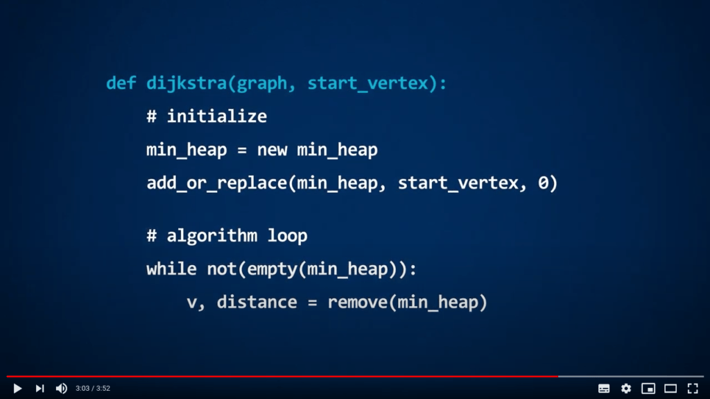
L’objectif de l’algorithme de Dijkstra est de trouver les chemins les plus courts entre une position de départ et tous les autres sommets dans un graphe pondéré. Pour implémenter cet algorithme en utilisant un tas min, il suffit d’ajouter les sommets comme clés, et les distances à la position de départ comme valeurs associées.
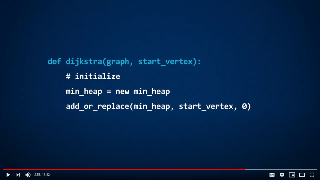
On peut simplement initialiser un tas min vide, et ajouter le sommet de départ avec une valeur de 0.
Ensuite, on effectue une boucle tant que le tas min n’est pas vide.
On retire une paire (clé, valeur) du tas min, ce qui renverra un sommet et sa distance.
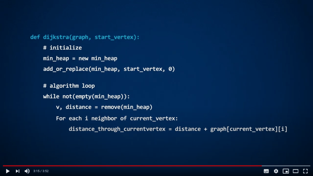
Ensuite, on examine chaque voisin du sommet que l’on vient de retirer du tas min. Les distances sont mises à jour en ajoutant la distance stockée et le poids de l’arête correspondant à ce voisin.
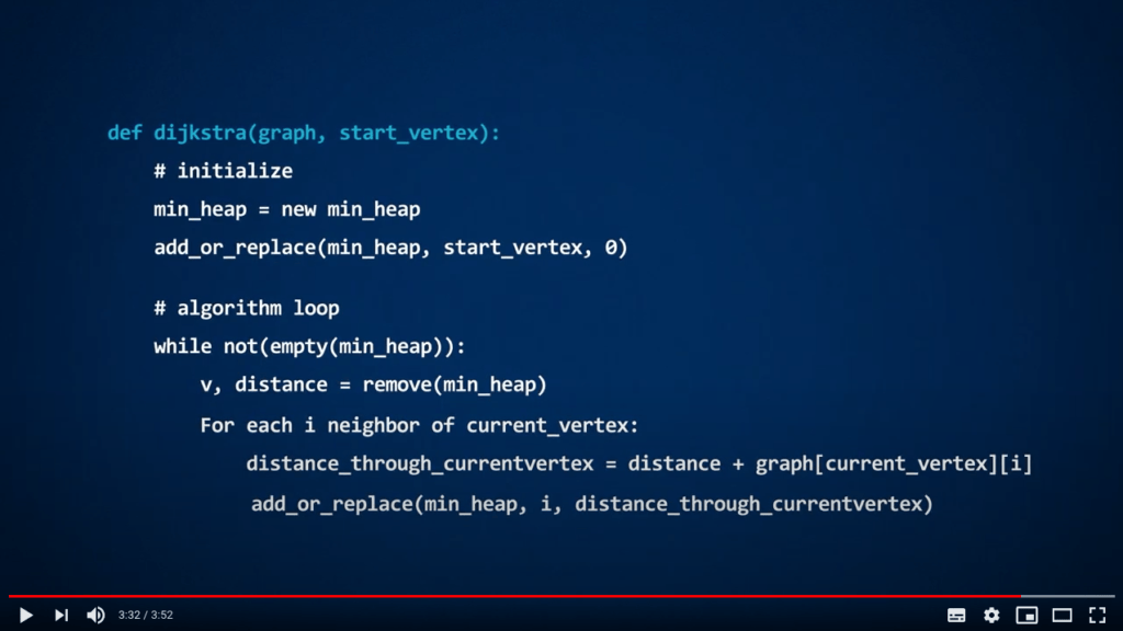
Puis, on utilise add_or_replace(...) pour l’entrée correspondant à ce voisin dans le tas min, ce qui mettra automatiquement à jour la distance avec la valeur minimale, si nécessaire.
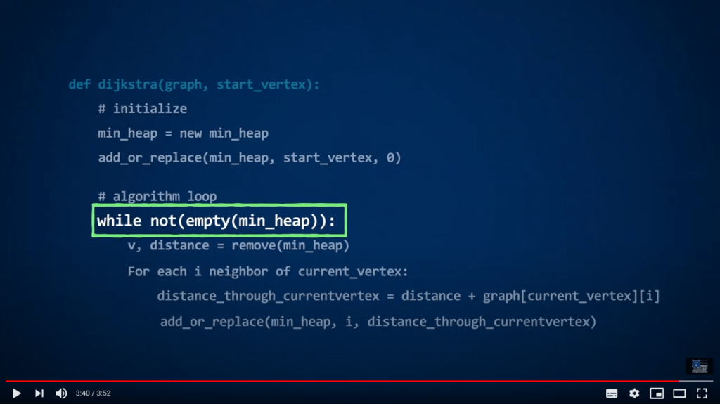
Ce processus continue jusqu’à ce que le tas min soit vide, ce qui correspond au fait que tous les sommets ont été visités.
Voilà pour aujourd’hui, à bientôt pour la prochaine vidéo !
Voici quelques remarques importantes sur cette vidéo :
-
Dans cette vidéo, nous avons utilisé les termes “clé” (l’élément que nous voulons stocker) et “valeur” (son importance dans le tas). D’autres terminologies existent ! L’aspect important est que
remove(...)doit retourner l’élément minimum de la structure. Attention à la manière dont ce minimum est calculé ! -
Dans la vidéo, une implémentation possible de l’algorithme de Dijkstra est présentée, utilisant une fonction appelée
add_or_replace(...). Ici, nous expliquons simplement ce que fait cette fonction, mais nous ne fournissons pas son code. Lorsque vous implémenterez l’algorithme en Python, vous devrez créer une telle fonction ou réfléchir à une autre solution.
Pour aller plus loin
2 — Une implémentation naïve d’un tas min utilisant une liste
Une manière simple (mais assez inefficace) d’implémenter un tas min est d’utiliser une liste pour stocker des paires (clé, valeur).
Dans cette section, nous montrons comment créer un tas min comme ça.
Créons une classe pour notre tas min naïf. Cela permettra de créer un nouveau tas min et d’effectuer des opérations dessus :
Dans le constructeur de notre classe, nous créons un attribut pour stocker les éléments. Dans cette implémentation, nous créons simplement une liste vide :
Maintenant, nous devons définir les deux méthodes présentées dans la vidéo : add_or_replace(...) et remove(...).
Commençons par la première.
Nous allons procéder comme suit :
- Tout d’abord, nous vérifions si la liste contient la clé que nous voulons ajouter.
- Si c’est le cas, et que la valeur associée est supérieure à la valeur que nous voulons ajouter, nous la supprimons.
- Enfin, nous ajoutons la paire
(clé, valeur)que nous voulons stocker si nécessaire.
Cela correspond au code suivant :
En termes de complexité, cette implémentation doit parcourir toute la liste des éléments. Comme cette liste peut contenir jusqu’à $n$ éléments, où $n$ est le nombre de sommets dans le graphe, elle est de complexité $O(n)$.
Maintenant, pour retirer un élément, comparons simplement les valeurs de tous les éléments dans la liste, et retournons celui avec la plus petite valeur :
En termes de complexité, cette implémentation est de complexité $O(n)$ pour les mêmes raisons que celles mentionnées ci-dessus.
Testons notre tas min en utilisant le même exemple que dans la vidéo :
Voici la sortie que nous obtenons :
Vous voulez essayer par vous-même ?
Voici une implémentation de cette classe.
Si vous souhaitez l’utiliser dans vos programmes, n’hésitez pas à la copier dans un répertoire pyrat_workspace/utils.
3 — Une meilleure implémentation
Eh bien, $n$ opérations pour ajouter un élément, et $n$ opérations pour en retirer un, ce n’est pas très efficace.
Ainsi, la complexité de l’implémentation naïve de add_or_replace(...) a un impact sur les performances du code et la consommation d’énergie.
Il est assez évident que nous pouvons faire mieux, par exemple en gardant la liste triée, de sorte que remove(...) ait simplement à retourner le premier élément.
Avec une telle adaptation, remove(...) aurait une complexité de $O(1)$, au prix d’un surcoût computationnel dans add_or_replace(...).
En pratique, il existe des solutions encore meilleures, basées sur des structures de données plus complexes.
En Python, nous pouvons utiliser une bibliothèque appelée heapq.
Cette bibliothèque fournit deux méthodes :
heappush(...), qui ajoute un élément au tas min.heappop(...), qui retire l’élément minimum du tas min.
Voyons ce qui se passe avec le même exemple que dans la vidéo :
Semble assez similaire à ce que nous avions avant, n’est-ce pas ? Eh bien, voyons la sortie :
Ce que fait cette bibliothèque, c’est qu’elle retourne l’élément minimum parmi ceux qui ont été ajoutés.
Ici, les éléments sont des paires, donc heapq déterminera quelle paire est la plus petite en vérifiant leur contenu dans l’ordre lexicographique, i.e., le premier élément de la paire, puis le second.
Dans l’exemple ci-dessus, les comparaisons sont faites sur "A", "B" et "C" plutôt que sur les valeurs numériques, qui ne sont utilisées qu’en cas d’égalité sur la première entrée.
Corrigeons cela en inversant les clés et les valeurs :
Voici la sortie que nous obtenons maintenant :
Mieux déjà, mais il semble que heappop(...) ne réalise pas d’opération de remplacement lorsque la clé existe déjà.
En effet, il se contente d’ajouter des éléments à une structure, sans réelle notion de “clés” ou de “valeurs”.
Il a simplement la propriété de retourner l’élément minimum lorsqu’on le demande.
Alors, comment peut-on utiliser cela pour implémenter l’algorithme de Dijkstra ? En fait, il est possible d’adapter simplement l’algorithme vu dans le cours. En effet, lorsqu’un sommet est extrait du tas min, vous savez que vous avez trouvé le chemin le plus court vers ce sommet. Ainsi, si vous extrayez plus tard le même sommet, vous savez qu’il s’agit d’un chemin plus long, et vous pouvez donc simplement l’ignorer !
Eh bien, cela ne nous dit pas si cette solution est meilleure que la solution naïve.
En réalité, heapq est un tas binaire, et les opérations heappush(...) et heappop(...) ont une complexité de $O(log_2(n))$, ce qui est inférieur à $O(n)$.
Nous donnons plus de détails ci-dessous si vous le souhaitez.
4 — Implémentation utilisant un arbre binaire équilibré
4.1 — Définitions
Commençons par quelques définitions. Vous devriez déjà savoir ce qu’est un arbre, et ce que nous appelons sa racine. Un sommet dans un arbre est un “nœud” s’il a des voisins plus éloignés de la racine de l’arbre (que nous appelons enfants). Sinon, c’est une “feuille”.
La “profondeur” d’un arbre est la longueur du plus long chemin le plus court partant de la racine. Un arbre est “équilibré” si tous ses chemins les plus courts partant de la racine ont la même longueur, $\pm 1$.
4.2 — Le modèle d’arbre
Au lieu d’utiliser une liste, il est proposé d’utiliser un arbre binaire équilibré avec les propriétés suivantes :
-
Chaque nœud de l’arbre est associé à un couple (clé, valeur). Cette propriété permet de lier l’arbre aux éléments à stocker/extraire.
-
Chaque nœud parent a deux enfants, sauf si le nombre total d’éléments dans la structure est impair, auquel cas un seul nœud a un seul enfant et tous les autres en ont deux.
-
L’arbre est équilibré. Cette propriété garantit que l’arbre ne prend pas une forme similaire à une longue chaîne, en devenant une sorte de liste, perdant ainsi tout l’intérêt d’utiliser des arbres.
-
La valeur d’un parent est toujours inférieure à celle de ses enfants. Cette propriété essentielle garantit que le nœud de valeur minimale est toujours à la racine.
Information
Des arbres ternaires/quaternaires/etc. pourraient également être envisagés (ce qui change le nombre d’enfants). À mesure que le nombre d’enfants augmente, la complexité de l’opération d’insertion diminue, mais la complexité de l’extraction augmente.
4.3 — Création
Pour initialiser une telle structure de priorité, il suffit de retourner un arbre vide.
4.4 — Insertion
Pour insérer un couple (clé, valeur) dans l’arbre, procédez comme suit :
- Le couple
(clé, valeur)est ajouté à la fin de l’arbre, i.e. :
- Si tous les nœuds parents ont deux enfants, une feuille de profondeur minimale est transformée en parent de ce nœud.
- Si un nœud parent n’a qu’un seul enfant, il est ajouté comme second enfant de ce nœud.
-
Si la valeur de ce nouveau nœud est inférieure à celle de son parent, les couples
(clé, valeur)du nœud et de son parent sont échangés. -
On continue en remontant dans l’arbre autant que nécessaire.
Puisque nous ne faisons que remplacer des éléments dans l’arbre par des éléments de valeurs plus petites, l’arbre résultant conserve les propriétés énoncées si l’arbre d’origine les avait.
4.5 — Extraction
Pour extraire un élément, procédez comme suit :
-
Le couple
(clé, valeur)associé à la racine de l’arbre est retourné. -
On le remplace par une feuille de profondeur maximale de l’arbre.
-
Si la nouvelle racine a une valeur supérieure à l’une de ses enfants, le couple
(clé, valeur)est échangé avec l’enfant de plus petite valeur. -
On recommence en descendant autant que nécessaire.
Ici encore, il est facile de vérifier que l’arbre résultant respecte les propriétés énoncées si l’arbre de départ les respectait également.
4.6 — Complexité
La complexité des opérations d’insertion et d’extraction nécessite d’aller de la racine à une feuille de profondeur maximale dans le pire des cas. L’arbre étant binaire, cela représente $log_2(n)$ opérations, où $n$ est le nombre d’éléments dans la structure. Nous sommes donc beaucoup moins complexes qu’avec une implémentation naïve utilisant une liste (où le nombre d’opérations était au moins linéaire en $n$).
Pour aller plus loin
-
Une liste plus complète des structures de données de priorité.
-
L’algorithme de parcours A* est quelque chose que vous pourriez vouloir essayer dans le projet.